 風況解析実行]をクリックすると、
風況解析ダイアログボックスが表示されます。
風況解析実行]をクリックすると、
風況解析ダイアログボックスが表示されます。Airflow Analyst > 操作ガイド Operation Guide > 解析プロジェクト Analysis project
計算格子を作成した後、 以下の手順で解析設定データを出力し、風況解析ソルバーを実行します。
Once you have created a computational grid, output the analysis setting files and execute the wind analysis solver as follows.
解析ツールバーの[風況解析実行]をクリックすると、
風況解析ダイアログボックスが表示されます。
On the Analysis toolbar, click [Run Solver]
to display the Wind Analysis dialog box.
最初から計算する場合は、こちらを選択します。
To compute from the beginning, choose this mode.
前回の計算結果データを引き継いで計算する場合は、こちらを選択します。
継続計算は、前回の計算結果データ(各種.datファイル)が作業ディレクトリに残っている場合のみ可能です。
(※計算結果データファイルは実行時に上書きされます。)
To carry on computing with the previous computation result data, choose this mode.
This mode is available only when the previous computation result data files remain in the working directory.
(* Those data files will be overwritten during the computation.)
ソルバーで行う計算の回数を『ステップ』という単位で設定します。
ソルバーは、時間とともに進展する流れを計算します。
流れが始まる初期状態から流れが発達し、同じような流れのパターンが繰り返し発生する定常状態になるまで、
通常25,000ステップ程度の計算が必要になります。
(実際には、計算条件によってこれらの数値は増減します。)
Enter the total number of calculations of the solver in the unit of "step".
The solver computes flows that evolve over time.
A flow evolves from the initial state where the flow begins, to the steady state where the similar flow pattern repeats occurs,
and usually it takes about 25,000 steps of calculations.
(Actually, this number will increase or decrease depending on the conditions of the computation.)
総ステップ数が多いほどシミュレーションは長くなり、 計算にかかる時間も長くなります。
As the total number of calculation steps increases, the simulation time becomes longer, and it takes a longer time to complete the computation.
計算結果をファイルに出力するステップ間隔を設定します。
1ステップ毎に格子全体の瞬間風況が算出されますが、その全てをファイルに保存するとデータ量が膨大になります。
程よい間隔で出力することがデータ容量の節約や可視化時の見やすさにつながります。
通常100ステップに1回の割合で保存すれば、可視化に適した出力になります。
Enter the step interval for outputting the calculation result to the files.
The instantaneous wind condition of the entire grid is calculated every step, but if all of them are saved in the files, the data volume becomes huge.
Outputting at moderate intervals leads to saving of data capacity and improving the visualization.
Usually, if they are saved every 100 steps, it will be suitable for visualization.
総ステップ数"25,000"、保存間隔"100"の場合、可視化の際には25,000 / 100 = "250"フレームのアニメーションとなります。
If the total step number is "25,000" and the storage interval is "100", visualization will be 25,000 / 100 = "250" frames animation.
時間平均データ(tave)の計算を開始するステップ番号を設定します。
Enter the step number to start calculation of the time averaged data (tave).
このチェックボックスをオンにすると、統計開始ステップは自動的に設定されます。 自動設定の場合、新規計算モードでは総ステップ数の半分となり、継続計算モードでは最初のステップとなります。
If you select this check box, the statistics start step will be set automatically. In the case of automatic setting, the value is half of the total number of steps in the "New" mode, and is the first step in the "Continue" mode.
流入面においては、べき指数に従った曲線(風速プロファイル)で風速が設定されます。
一般的に、市街地など起伏の大きな場所でのべき指数は"3"程度、平坦地や海など起伏の無いところのべき指数は"7"程度の値が採用されています。
On the inlet section, wind speed is set by a curve (wind speed profile) according to power index.
Generally, the power index of about "3" is adopted for places with large undulations such as urban areas,
and about "7" for flat areas or those with no undulations such as the ocean.
気象モデルデータから境界値を取得する場合は、
気象モデルデータ内に格納されている風速の鉛直分布に沿って流入風速が作成されます。
ただし、気象モデルの最下層から地面までの風速については、
直線的な補間ではなくここで指定したべき指数を用いて曲線的に補間しています。
なお、地表面では必ず風速が"0"となります。
When acquiring the boundary value from the weather model data,
the inflow wind speed is created along the vertical distribution of the wind speed stored in the weather model data.
But as for the wind speed from the lowermost layer of the weather model to the ground,
interpolation is performed in a curved manner using the power index specified here, instead of the linear interpolation.
In addition, the wind speed is always "0" on the ground surface.
1ステップ当たりの無次元時間の間隔を設定します。 通常はデフォルト値の0.002を設定してください。
Enter the non-dimensional time interval per step. Normally, set the default value "0.002".
風の流れの計算だけを行う場合は、こちらを選択します。
Select this mode to compute only airflow.
風の流れと拡散の計算を行う場合は、こちらを選択します。
Select this mode to compute airflow and diffusion.
拡散計算を行う際は、 計算格子設定ダイアログボックスの[物体レイヤー]で指定したフィーチャークラスにおいて、 発生源の形状を表すフィーチャーを作成し、[物体種別コード]で指定したフィールドに"5"を設定する必要があります。
When performing the diffusion computation, edit the feature class specified by [Object Layer] in the Grid Settings dialog box to create features representing shapes of the source, and set "5" for the field of them specified by [Object Type Code].
計算を安定させるため、ソルバーは一時的に計算格子の流出口側に平坦な格子を加えて計算を行います。 この袖領域メッシュはソルバーの自動処理によって追加され、計算結果データからは除去されて出力されるので、 実際にユーザがこの袖領域を目にすることはありません。
To stabilize the computation, the solver adds a flat temporary mesh to the outlet side of the computational grid and compute it. This sleeve area mesh is added by automatic processing of the solver, and it is removed from the computation result data when outputting, so you will not actually see this sleeve area.
通常は、デフォルト値を使用します。
([袖領域の格子数]="10"、[袖領域パラメーター]="1.3")
計算が途中で発散する場合は、これらの値を増加させることで発散を抑制できることがあります。
Normally, use the default values.
([Number of Sleeve Meshes]="10", [Sleeve Parameter]="1.3")
If the computation diverges in the middle, divergence can be suppressed by increasing these values.
大気の安定度を-1.0~1.0の数値で指定します。
-1.0に近いほど強不安定、0.0は中立、1.0に近いほど強安定、となります。
Enter the atmospheric stability with a numerical value of -1.0 to 1.0.
The closer to -1.0 the stronger the instability, 0.0 the neutral, the closer to 1.0 the more stable it becomes.
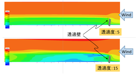
樹木や防風ネットのような、一部の風を通過させる物体(透過壁)を模擬する際に使用します。
It is used to simulate objects (permeable walls) that allow some wind to pass like trees and windbreak nets.
この値が"0"の場合、透過壁は抵抗なく風を通す状態となります。 数値が大きくなるほど抵抗は大きくなります。
If this value is set to "0", the permeable walls pass the wind without resistance. The resistance increases as the number increases.
この設定は、計算格子設定ダイアログボックスで選択された[物体レイヤー]において、 [物体種別コード]フィールドの値が"2"(透過壁)のフィーチャーに適用されます。
This setting is applied to features whose [Object Type Code] field value is "2" (permeable wall) in [Object Layer] selected in the Grid Setting dialog box.
計算格子設定ダイアログボックスの[回転]で指定した風向のみ、データ作成やソルバー実行するモードです。
This mode is to create data and run the solver only on the wind direction specified by [Rotation] in the Grid Settings dialog box.
現在の格子設定で基準点を中心に格子を回転させ、 16風向リストのうち選択された風向の格子データを順番に作成し、 風向別の作業ディレクトリに出力するモードです。
Rotating the grid centering around the reference point in the current grid setting, it creates grid data of the selected directions on the list, and outputs each one separately in the working directory.
現在の作業ディレクトリ内に、00_N、01_NNE、02_NE…14_NNWのような風向別の作業ディレクトリが自動的に作成されます。 同じ条件で複数の風向のシミュレーションを行いたい場合に便利です。
Working directories by directions such as 00_N, 01_NNE, 02_NE ... 14_NNW are automatically created in the current working directory. This is useful when simulating multiple inflow directions under the same conditions.
風向別データ出力後にソルバーは実行されません。 後で個別に実行するか、後述のバッチ処理で実行してください。
The solver will not run after outputting data by direction. Run it individually later, or by batch processing to be described later.
すぐにソルバーを実行せず、解析設定データファイルの作成のみを行う場合は、このチェックボックスをオンにします。 作成した計算格子を確認したい場合や、ソルバーを別の時間に実行したい場合、複数ケースの計算をバッチ処理で実行したい場合などに使用します。
Select this check box if you do not run the solver immediately and only create the analysis setting files. It is used if you want to check the computational grid you have created, to run the solver at different time, or to solve multiple cases by batch processing.
ソルバーを実行したい場合は、このチェックボックスをオフにしてください。
If you want to run the solver, clear this check box.
このチェックボックスをオンにすると、データ作成する前に、 作業ディレクトリ内の既存の解析データファイル群を別のフォルダに保存します。
Select this check box to save existing analysis data files in the working directory to another folder before creating data.
現在のソルバー設定をプロジェクトに登録します。
Apply the current solver settings in the project.
クリックすると、ソルバーを実行します。 必要な解析設定データが未作成または再作成する場合は、まずデータ作成処理が行われます。 格子サイズが大きい(格子点数が多い)ほど時間がかかります。
Click to run the solver. If the required analysis setting files are not created or need to be re-created, data creation processing is performed first. The larger the grid size (the larger the number of grid points), the longer it takes.
解析設定ファイル群の作成が完了すると、ソルバーが起動します。 ソルバーによる計算は、格子サイズが大きい・ステップ数が多いほど時間がかかります。 計算中はCPU負荷の高い状態が継続し、格子サイズが大きい場合は多大なマシンパワーを要します。
When the anaylsis setting files have been created, the solver starts running. Computation by the solver takes a lot of time as the grid size is large or the number of calculation steps increases. During the computation, the CPU load continues to be high, and if the grid size is large, a lot of machine power is required.
ソルバーの実行後には、現在の解析プロジェクトが自動的に別名ファイルとして保存されます。
After running the solver, current analysis project is automatically saved as a file with a different name.
このダイアログボックスを閉じます。
Click to close the dialog box.
ソルバー実行中は、下図のようなウインドウに計算進捗が表示されます。
While the solver is running, the computation progress is displayed in the window as follows.
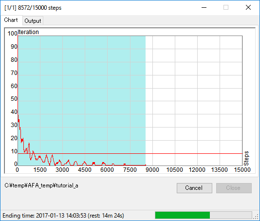
ソルバーの計算進捗がグラフ表示されます。 進捗状況を示す色付きの面がグラフの右端まで進むと計算完了です。
Current computation progress of the solver is displayed as a chart. The computation is completed when the colored area indicating current progress goes to the right end of the chart.
| 状況 | 面の色 |
|---|---|
| Situation | Fill Color |
| 計算中 In Progress | 薄水色 Pale Blue |
| 計算完了(成功) Completed Successfully | 白色 White |
| 計算終了(中止・失敗) Stopped (Cancelled / Failed) | 橙色 Orange |
| 計算終了(発散) Diverged | 薄橙色 Light Orange |
グラフの赤い線は、計算の反復回数を示しています。
101回から開始し、計算の進展に従って徐々に減って10以下になれば
順調に計算が収束していることを示します。
反復回数が小さいことが計算結果の精度が高いことを示すわけではありません。
しかし、数千ステップの計算を行っても反復回数が大きい場合、
計算が順調に進展していない可能性があり、
計算格子の設定を見直す必要があることを示唆しています。
The red line in the chart shows the number of iterations of the calculation.
Starting from 101 times, gradually decreasing as the computation progresses, and when it becomes 10 or less,
it indicates that the computation has successfully converged.
Small number of iterations does not mean that the accuracy of the computation result is high.
But if the iteration number is large even when the thousands of calculation steps are performed,
the computation may not progress smoothly,
it suggests that you need to reconsider the settings of the computational grid.
グラフの青い線は、二乗平均平方根誤差(Root-mean-square error)を示しています。
The blue line in the chart shows the root-mean-square error.
グラフのデータは作業ディレクトリに"processlog.csv"として出力されます。
The data of the chart will be exported to the working directory as "processlog.csv".
ソルバーから出力されたメッセージが表示されます。 このメッセージは作業ディレクトリに"processlog.txt"として出力されます。
The messages output from the solver are displayed. These messages will be exported to the working directory as "processlog.txt".
クリックすると、グラフをPNG形式の画像ファイルに出力します。
Click to export the image of the chart to a PNG file.
クリックすると、途中で計算を中止します。再開はできません。
Click to cancel the computation. It cannot be restarted.
計算終了後にクリックすると、この画面を閉じます。
Click to close the window after the computation has finished.
反復計算において解が収束せず発散してしまうと、 その時点で計算を終了し、警告メッセージが表示されます。 この場合、計算格子やソルバー設定を修正し、最初から計算をやり直す必要があります。
If the solution does not converge and diverges in the iterative calculations, the computation is terminated at that point, and a warning message is displayed. In this case, it is necessary to revise the computational grid and solver settings, and retry the computation from the beginning.
複数ケースの計算を夜間など計算機の空いている時間にまとめて実行したい場合、 先に解析用データファイル群を作成しておき、後でソルバーをバッチ処理で実行できます。
If you want to compute multiple cases collectively at free time such as nighttime, you can create the analysis data files first, and run the solver later by batch processing.
Airflow Analystで解析用データファイルを出力すると、同じ作業ディレクトリに"solver_monitor.bat"が作成されます。 このファイルをダブルクリックすると、SolverMonitor.exeが起動します。
When you output the analysis data files by Airflow Analyst, "solver_monitor.bat" is created in the same working directory. Double click this file and SolverMonitor.exe will start up.
または直接、Airflow Analystのインストール先 (デフォルトでは"C:\Program Files (x86)\ENGIS\AirflowAnalyst\")にある"bin\SolverMonitor.exe"を起動します。
Or start "bin\SolverMonitor.exe" in the Airflow Analyst install directory.
Airflow Analystのインストール先にあるソルバー情報ファイル(solvers_xx\solvers_xx.xml)のパスを設定します。
("_xx"の部分はバージョンによって異なります)
Enter the absolute path of the "solver info file" (solvers_xx\solvers_xx.xml) in the Airflow Analyst install directory. (The "_xx" part depends on the edition)
ソルバーを実行する作業ディレクトリと、計算ステップ数などを設定します。
複数行設定すれば、バッチ処理となります。
設定を追加したい場合は、テーブルの上に作業ディレクトリのフォルダアイコンをドラッグ・ドロップするか、
[Add Data Directory]をクリックします。
設定を削除したい場合は、行の左端をクリックして選択状態にして、Deleteキーを押下します。
Specify the working directory to run the solver, and the number of calculation steps.
If you set multiple rows, it will be batch processing.
To add settings, drag and drop folder icons of working directories on the table,
or click [Add Data Directory].
To delete settings, click the left end of the rows to select them, and press the Delete key.
ソルバーの実行結果が表示されます。
The execution result of the solver will be displayed.
解析設定データが入っている作業ディレクトリの絶対パスを入力します。
Enter the absolute path of the working directory containing the analysis setting files.
para*.datファイルに設定されている計算ステップ数です。(変更可)
The number of calculation steps that is set in the para*.dat file. (Editable)
para*.datファイルに設定されている計算結果データ記録間隔です。(変更可)
The interval of recording the calculation result that is set in the para*.dat file. (Editable)
オンの場合は継続計算、オフの場合は新規計算を実行します。(変更可)
Select this check box for the continuing computation, or clear for the new computation. (Editable)
クリックして作業ディレクトリを選択し、テーブルに追加します。
Click to add a working directory to the table.
クリックすると、解析設定テーブルの上から順に、ソルバーによる処理が実行されます。 実行中はソルバー進捗ウインドウが表示されます。
Click to start processing by the solver, in order from the top of the table. The solver progress window is displayed during execution.