Airflow Analystクイックスタートチュートリアル(旧版)
Airflow Analyst Quick Start Tutorial (Old version)
本チュートリアルでは、Airflow AnalystのセットアップからArcScene上での計算格子作成、ソルバー実行、計算結果の可視化まで、
一連の操作手順を案内します。
In this tutorial, we will guide you through a series of operation procedures
from setting up Airflow Analyst to creating computational grid on ArcScene, running airflow solver, and visualizing the computation results.
Airflow Analystのセットアップ
Set up Airflow Analyst
事前準備
Advance Preparation
- Airflow Analyst (バージョン 1.6) は、ESRI ArcGIS 10.5~10.6.1のエクステンション(拡張機能)として、ArcScene上で動作します。
Airflow Analystをインストールする前に、ArcGIS 10.5~10.6.1と3D Analystをインストールし、利用可能な状態にしておいてください。
- Airflow Analyst (Version 1.6) operates on ArcScene as an extension of ESRI ArcGIS 10.5 - 10.6.1.
Before installing Airflow Analyst, install ArcGIS 10.5 - 10.6.1 and 3D Analyst and make them available.
- Airflow Analystの動作には、Microsoft Visual C++のランタイム・ライブラリ"Microsoft Visual C++2015 Redistributable (x86)"が必要です。
下記サイトから、
インストールプログラム"vc_redist.x86.exe"をダウンロードして、実行してください。
- Airflow Analyst requires the Microsoft Visual C ++ runtime library "Microsoft Visual C ++ 2015 Redistributable (x86)".
From the following site,
download the installation program "vc_redist.x86.exe", and then run it.
Microsoft Visual C++ 2015 Redistributable Update 3
- Windows 7の場合は、Microsoft .Net Framework 4.5以上をインストールしてください。
- For Windows 7, install Microsoft .Net Framework 4.5 or higher.
- ハードウェアキー(Sentinel HASPキー)が必要なエディションの場合は、ハードウェアキーのドライバーソフトウェアが必要です。
下記サイトから、
インストールプログラム"Sentinel HASP/LDK - Windows GUI Run-time Installer (Version 7.53)"をダウンロードして、実行してください。
インストール後に、ハードウェアキーをコンピューターのUSBポートに差し込んでください。
- For editions that need a hardware key (Sentinel HASP key), the driver software of the hardware key is required.
From the following site,
download the installation program of "Sentinel HASP / LDK Windows GUI Run -time Installer (Version 7.53)", and then run it.
After the installation, insert the hardware key into the USB port of the computer.
Sentinelのダウンロードサイト
Sentinel Download Site
- アンチウィルスソフトの動作によって、セットアップが阻害され正常に起動しないことがあります。
その場合、一時的にアンチウィルスソフトを無効にして、再度セットアップしてください。
- Because of the operation of the antivirus software, setup may be disturbed and it may not start normally.
In that case, temporarily disable anti-virus software and set it up again.
Airflow Analystのインストール
Installing Airflow Analyst
- インストール作業は、管理者権限を持つユーザで実行してください。
- Perform installation work as a user with administrator authority.
- Airflow AnalystセットアップDVD内の、またはAirflow Analyst配布サイトからダウンロードした
"Setup.exe"をダブルクリックして起動します。
- Double-click "Setup.exe" in the Airflow Analyst setup DVD or downloaded from the from Airflow Analyst distribution site to start it.
- Airflow Analystセットアップウィザードの進行に従って、インストール作業を行います。
- Follow the progress of the Airflow Analyst Setup Wizard and perform the installation work.
Airflow Analystエクステンションの有効化
Activating the Airflow Analyst Extension
- Windowsのスタートメニューの[ArcGIS > ArcScene]をクリックし、ArcSceneを起動します。
- On the Windows start menu, Click [ArcGIS > ArcScene] to start ArcScene.
- ArcSceneのメインメニューの[Customize (カスタマイズ) > Extensions (エクステンション)]をクリックします。
- On the ArcScene main menu, Click [Customize > Extensions].
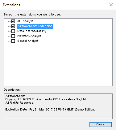
- [Extensions (エクステンション)]ダイアログボックスで、[Airflow Analyst Extension]をオンにします。
- In the [Extensions] dialog box, select [Airflow Analyst Extension].
Airflow Analystツールバーの表示
Showing the Airflow Analyst Toolbar
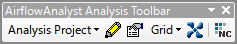
- Airflow Analystは、[Airflow Analyst Analysis Toolbar (解析ツールバー)]と、
[Airflow Analyst Visualization Toolbar (可視化ツールバー)]の2種類のツールバーから操作します。
- Airflow Analyst operates from two toolbars:
[Airflow Analyst Analysis Toolbar] and [Airflow Analyst Visualization Toolbar].

- これらのツールバーが画面に表示されていない場合は、
ArcSceneのメインメニューの[Customize (カスタマイズ) > Toolbars (ツールバー)]でそれぞれをオンにして表示します。
- If these toolbars are not displayed on the screen,
on the ArcScene main menu, click [Customize > Toolbars], and select them.
ライセンスの更新
License Update
- ライセンスの確認
- Confirming the license
Airflow Analystのライセンスには有効期限が設定されています。
Airflow Analystエクステンションは、それを過ぎると使用できなくなります。
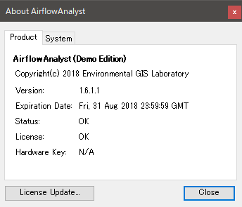
ライセンスの有効期限は、解析ツールバーの[Analysis Project (解析プロジェクト) > About Airflow Analyst (Airflow Analystについて)]で確認できます。
The Airflow Analyst license has an expiration date.
The Airflow Analyst extension will be unusable after that.
To check the expiration date of the license, click [Analysis Project > About Airflow Analyst] on the Analysis Toolbar.
- ライセンスの更新
- Updating the license
ライセンスが期限切れの場合は、新しいAirflow Analystライセンスファイル(.afl)を入手し、以下の手順で更新してください。
If the license has expired, obtain a new Airflow Analyst license file (.afl) and update it with the following procedure.
- 解析ツールバーの[Analysis Project (解析プロジェクト) > About Airflow Analyst (Airflow Analystについて)]をクリックします。
- On the Analysis Toolbar, click [Analysis Project > About Airflow Analyst].
- [About Airflow Analyst (Airflow Analystのバージョン情報)]ダイアログボックスで、[License Update (ライセンス アップデート)]をクリックします。
- In the [About Airflow Analyst] dialog box, click [License Update].
- ファイル選択ダイアログボックスで、入手したライセンスファイルを指定してください。
- In the file selection dialog box, select the license file you obtained.
- [About Airflow Analyst (Airflow Analystのバージョン情報)]ダイアログボックスに、有効期限の日付と"License (ライセンス) : OK"が表示されれば更新完了です。
- If the expiration date and "License (OK)" are displayed in the [About Airflow Analyst] dialog box, update is completed.
ハードウェアキー
Hardware key
- エディションによっては、Airflow Analyst専用のハードウェアキーが必要となります。
- Depending on the edition, a hardware key is required to activate Airflow Analyst.
- [About Airflow Analyst (Airflow Analystのバージョン情報)]ダイアログボックスで、
"Hardware Key (ハードウェアキー) : N/A"と表示されている場合は必要ありません。
- It is not necessary if "Hardware Key (N / A)" is displayed in the [About Airflow Analyst] dialog box.
- 必要な場合は、ハードウェアキーをコンピューターのUSBポートに差し込んでからArcSceneを起動してください。
- If necessary, plug in the hardware key to the USB port of your computer, and start ArcScene.
Airflow Analystの準備は以上です。ここで一旦、ArcSceneを終了します。
The preparation of Airflow Analyst is over. Exit ArcScene once.
計算格子の作成
Create a computational grid
まず、シミュレーション範囲の計算格子を作成します。
First, create a computational grid in the area of simulation.
チュートリアル用地形・建物GISデータの準備
Preparing the terrain / buildings GIS data for tutorial
- Airflow Analystセットアップフォルダー内の"Tutorial"フォルダーを、コンピューターの任意のフォルダーにコピーします。
または、Airflow Analyst配布サイトからチュートリアル用データをダウンロードします。
- Copy the "Tutorial" folder in the Airflow Analyst setup folder to any folder on your computer.
Or download tutorial data from the Airflow Analyst distribution site.
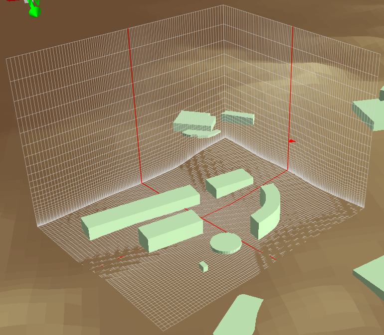
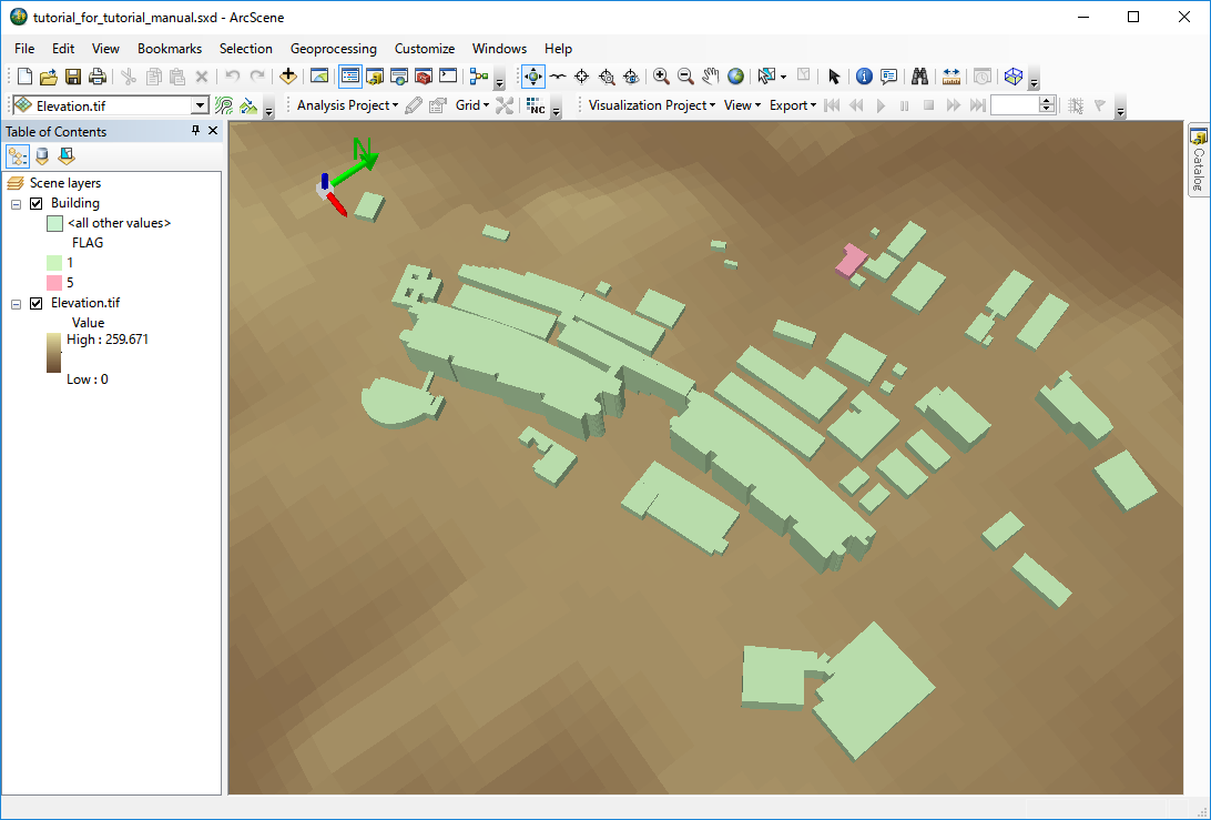
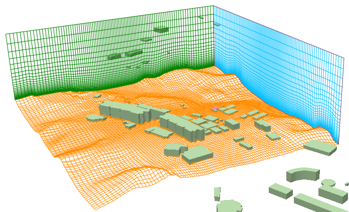
- "Tutorial"フォルダー内の"Tutorial.sxd"をダブルクリックします。
ArcSceneが起動し、地形と建物が3Dで表示されます。
- Double-click "Tutorial.sxd" in the "Tutorial" folder.
ArcScene will start up and the terrain and buildings will be displayed in 3D.
- 3D Analystツールバーの[
 Navigate (ナビゲート)]をクリックすると、
3Dシーン上でのマウス操作により視点を変更できます。
Navigate (ナビゲート)]をクリックすると、
3Dシーン上でのマウス操作により視点を変更できます。
- On the 3D Analyst Toolbar, click [Navigate],
you can change the viewpoint by moving the mouse on the 3D scene.
新規解析プロジェクト
New analysis project
- 解析ツールバーの[Analysis Project (解析プロジェクト) > New (新規)]をクリックします。
- On the Analysis Toolbar, click [Analysis Project > New].
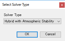
- ソルバーが変更可能なエディションの場合は、[Select Solver Type (ソルバータイプ選択)]ダイアログボックスが表示されます。
リストから"Hybrid with Atmospheric Stability (ハイブリッド 大気安定度対応)"を選択して[OK]をクリックしてください。
(評価版では表示されません。)
- If the edition allows you to change solvers, the [Select Solver Type] dialog box is displayed.
Select "Hybrid with Atmospheric Stability" and click [OK].
(It will not be displayed in the evaluation edition.)
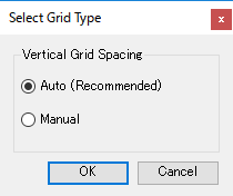
- [Select Grid Type (格子タイプ指定)]ダイアログボックスで、
"Auto (Recommended) (自動設定(推奨))"を選択し、[OK]をクリックします。
- In the [Select Grid Type] dialog box, select "Auto (Recommended)" and click [OK].
- フォルダー選択ダイアログボックスで、作業ディレクトリとするフォルダーを指定します。
この作業ディレクトリには、解析用データファイル群や計算結果データファイル群が格納されます。
- In the folder selection dialog box, select a folder to be the working directory.
This working directory will store analysis data files and computation result data files.
- 計算結果ファイルはサイズが数百MB~数GBと巨大になるため、
作業ディレクトリにするフォルダーは、容量に余裕があり高速にアクセスできるドライブに作成してください。
- Since the size of computation result files are huge, from several hundred megabytes to several gigabytes,
make a working directory on the drive with sufficient capacity and speedy access.
計算格子の設定
Setting the computational grid
- 解析ツールバーの[
 Grid Position (格子位置指定ツール)]をクリックします。
- On the Analysis Toolbar, click [Grid Position].
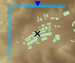
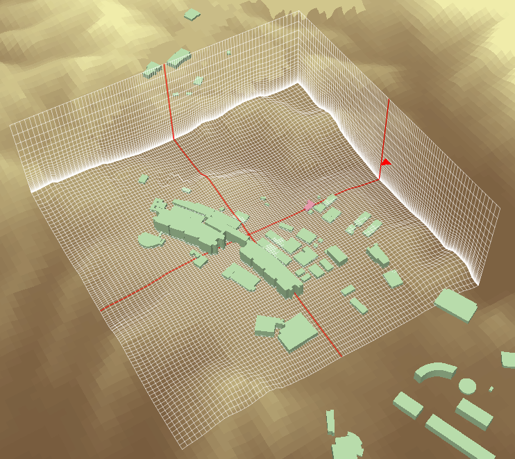
- ArcSceneの3Dシーン上で、計算領域の中心となる位置をクリックします。
本チュートリアルでは、下図の×印で指したあたりをクリックします。
中心位置は後から修正できるので、最初はおおよその位置で構いません。
何もない空間をクリックしても位置取得できないので、地形か建物の上をクリックしてください。
- On the 3D scene of ArcScene, click the center position of the analysis area.
In this tutorial, click at X in the following figure.
Since you can modify the center position later, the approximate position is acceptable at the beginning.
If you click on a space with nothing, you cannot get the position. So click on the terrain or buildings.
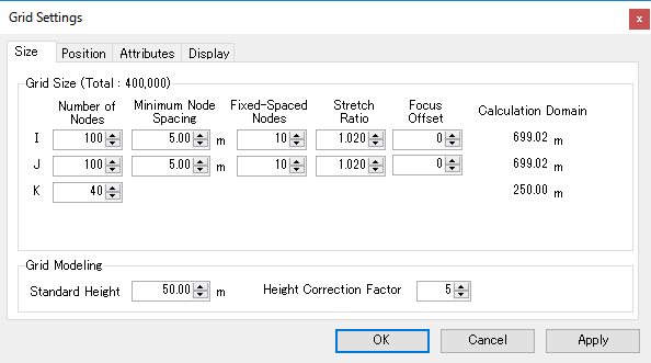
- マップに計算格子が描画され、[Grid Settings (計算格子設定)]ダイアログボックスが表示されます。
- A computational grid is drawn on the map, and the [Grid Settings] dialog box is displayed.
- ダイアログボックスの[Size (サイズ)]タブで、
[Minimum Node Spacing (基本格子幅)]の[I]と[J]をそれぞれ"5.00"に、[Standard Height (代表高さ)]を"50.00"にします。
- In the dialog box, on the [Size] tab, set [I] and [J] of [Minimum Node Spacing] to "5.00", and "Standard Height" to "50.00".
| [Minimum Node Spacing (基本格子幅) I] |
"5.00" |
| [Minimum Node Spacing (基本格子幅) J] |
"5.00" |
| [Standard Height (代表高さ)] |
"50.00" |
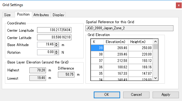
- [Position (位置)]タブをクリックし、[Rotation (回転(度))]を"0.00"にします。
計算風向は北を0度として時計回りで360度指定となるので、この場合は「北」からの風として設定されます。
- Click the [Position] tab, and set [Rotation] to "0.00".
The wind direction is specified as 360 degrees in clockwise direction with the north as 0 degrees, so in this case we set the north wind.
- [Attributes (属性)]タブをクリックし、[Base Elevation Layer (地表面標高レイヤー)]で"Elevation.tif"を選択します。
これにより、計算格子の底面となる地形データが設定されます。
- Click the [Attributes] tab, in the [Base Elevation Layer] list, select "Elevation.tif".
This sets the terrain data that will be the bottom of the computational grid.
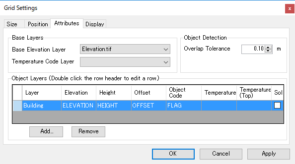
- [Object Layers (物体レイヤー)]欄の[Add (追加)]をクリックします。
- In the [Object Layers] group, Click [Add].
- [Object Data Field Settings (物体データ フィールド設定)]ダイアログボックスで、
下図のように設定し、[OK]をクリックします。
- In the [Object Data Field Settings] dialog box,
edit the settings as follows, and click [OK].
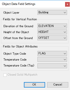
| [Object Layer (物体フィーチャーレイヤー)] |
"Building" |
| [Elevation of the Ground (地面の標高)] |
"ELEVATION" |
| [Height of the Object (物体の高さ)] |
"HEIGHT" |
| [Offset from the Ground (地面からのオフセット)] |
"OFFSET" |
| [Object Type Code (物体種別コード)] |
"FLAG" |
- 前項の設定により、物体レイヤーテーブルに、"Building"レイヤーが追加されます。
設定を修正する場合は、対象となる行の左端のセルをダブルクリックしてください。
削除する場合は、対象となる行を選択状態にして[Remove (削除)]をクリックしてください。
- By the setting in the previous section, "Building" layer is added to the object layer table.
To correct the setting, double-click on the leftmost cell of the target row.
To remove a object layer, select the target line and click [Remove].
- ダイアログボックスの[OK]をクリックして、格子設定を確定します。
下図のような格子が生成されます。
- Click [OK] in the dialog box to confirm the grid settings.
A grid is generated as follows.
- 格子設定を修正する際は、
解析ツールバーの[
 Grid Settings (格子設定)]をクリックすると、
[Grid Settings (計算格子設定)]ダイアログボックスが表示されます。
Grid Settings (格子設定)]をクリックすると、
[Grid Settings (計算格子設定)]ダイアログボックスが表示されます。
- To modify the grid settings,
click [Grid Settings] to show the [Grid Settings] dialog box.
以上で、シミュレーションに必要な計算格子設定は完了です。
With the above, the computational grid settings required for the simulation is completed.
解析プロジェクトの保存
Saving the analysis project
解析ツールバーの[Analysis Project (解析プロジェクト) > Save (保存)]をクリックして、
格子設定やソルバー設定を解析プロジェクトファイル(.afa)に保存します。
To save the grid settings and solver settings in the analysis project file (.afa),
click [Analysis Project > Save] on the Analysis Toolbar.
境界条件の設定(オプション)
Edit the boundary condition settings (optional)
必要に応じて、流入境界条件の設定ができます。
You can set the inlet boundary condition as necessary.
流入境界条件の設定
Setting inlet boundary condition
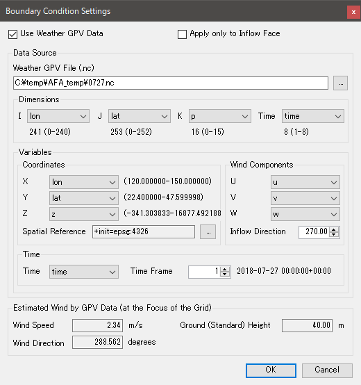
- 解析ツールバーの[Grid (格子) > Boundary Condition Settings (境界条件設定)]をクリックします。
[Boundary Condition Settings (境界条件設定)]ダイアログボックスが表示されます。
- Click [Grid > Boundary Condition Settings] on the Analysis Toolbar.
The [Boundary Condition Settings] dialog box appears.
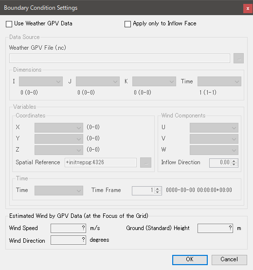
- 流入条件として気象モデルデータを参照する場合は、[Use Weather GPV Data (気象GPVデータから境界値を取得する)]をオンにして、
次項の「気象モデルデータの設定」を行ってください。
使わない場合はオフにして、[OK]をクリックしてください。
この場合、境界値は冪指数を使って算出されます。
- When using weather model data as inlet condition, select the [Use Weather GPV Data] check box,
and edit settings for weather model data in the next section.
Otherwise, clear the check box, then click [OK].
In this case, boundary values are calculated using power index.
気象モデルデータの設定
Setting the weather model data
- 日本周辺のメソ数値予報モデル GPV気圧面データ(MSM-P)の
NetCDF形式ファイル公開サイト
から、任意の年月日のNetCDF(.nc)ファイルをダウンロードします。
- Download any date of the netCDF (.nc) file from
the web site
publishing netCDF files of mesoscale numerical weather prediction model GPV data around Japan (MSM-P).
- [Weather GPV File (気象GPVデータファイル(MSM-P))]の[...]をクリックして、ダウンロードしたNetCDFファイルを選択します。
- Click [...] at the side of [Weather GPV File], and select the downloaded netCDF file.
- Data Source (データソース)欄で、下図のように設定します。
- In the [Data Source] group, edit the settings as follows.
| Dimensions (ディメンション) |
[I] |
"lon" |
| [J] | "lat" |
| [K] | "p" |
| [Time] | "time" |
| Coordinates (座標フィールド) |
[X] |
"lon" |
| [Y] | "lat" |
| [Z] | "z" |
|
Spatial Reference (空間参照) |
WGS84(+init=epsg:4326) |
| Wind Components (風速成分フィールド) |
[U] |
"u" |
| [V] | "v" |
| [W] | "w" |
|
Inflow Direction (流入口の方位) |
"270.0" |
| Time (時間フィールド) |
[Time (時間)] |
"time" |
|
[Time Frame (参照フレーム)] |
任意
any
|
- ダイアログボックスの下部にある[Wind Direction (風向)]の値を確認して、[OK]をクリックします。
- Confirm the value of [Wind Direction] at the bottom of the dialog box, and click [OK].
- 解析ツールバーの[Grid Settings (格子設定)]をクリックします。
- On the Analysis Toolbar, click [Grid Settings].
- [Grid Settings (計算格子設定)]ダイアログボックスで、[Position (位置)]タブの[Rotation (回転(度))]に、
先ほどの[Wind Direction (風向)]とほぼ同じ値を入力します。
- In the [Grid Settings] dialog box, click the [Position] tab.
In the [Rotation], enter nearly the same value as [Wind Direction] confirmed above.
風況解析ソルバーの実行
Run the wind analysis solver
計算格子の設定ができたら、風況解析ソルバーを実行します。
After setting the computational grid, run the wind analysis solver.
ソルバーの設定
Solver settings
- 解析ツールバーの[
 Run Solver (風況解析実行)]をクリックします。
- On the Analysis Toolbar, click [Run Solver].
- [Airflow Analysis (風況解析)]ダイアログボックスで、ソルバーの設定を編集します。
(下図は大気安定度対応ソルバーの場合です。)
- In the [Airflow Analysis] dialog box, edit solver settings.
(The following figure shows the case of the solver corresponding to atmospheric stability.)
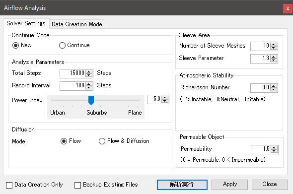
- Continue Mode (新規計算・継続計算)
新規に計算を行うか、既存の計算結果を引き継いで続きの計算を行うかを選択します。
本チュートリアルでは[New (新規)]を選択します。
Choose whether to start a new computation or to take over the existing computation result and compute continuously.
In this tutorial, select [New].
- Analysis Parameters (解析パラメーター)
- [Total Steps (総ステップ数)]
シミュレーション中の計算ステップ数を指定します。
本チュートリアルでは、"15000"ステップを指定します。
(※15,000ステップの計算は完了まで数時間かかります。数十分で済ませたい場合は"5000"ステップ程度で試してみてください。)
Set the total number of calculation steps in the simulation.
In this tutorial, set the value to "15000" steps.
It takes several hours for the simulation of 15,000 steps to complete.
If you wish to complete the simulation within several tens of minutes, set the value about "5000" steps.
- [Save Interval (保存間隔)]
計算結果をファイルに出力する間隔をステップ数で指定します。
本チュートリアルでは、"100"を指定します。
可視化の際には15,000/100=150フレームのアニメーションとなります。
Set the interval for outputting calculation results to a file in terms of the number of computational steps.
In this tutorial, set the value to "100".
When visualizing the analysis results, an animation with 15,000 / 100 = 150 frames will be created.
- [Power Index (べき指数)]
計算領域の地表の凹凸の状況に応じて設定します。
本チュートリアルでは、対象地が郊外の山間部であることから"5.0"を指定します。
Set a value according to the roughness of the surface in the area of analysis.
In this tutorial, set the value to "5" as the area is located in a suburban mountainous region.
- Diffusion (拡散)
気流の流れのみをシミュレートする場合は[Flow (気流場)]を、
拡散源から放出される物体の拡散現象もあわせてシミュレートする場合は[Flow & Diffusion (気流場・拡散場)]を選択します。
本チュートリアルでは、[Flow (気流場)]を選択します。
When simulating only the airflow, select [Flow].
When additionally simulating diffusion of a substance, select [Flow & Diffusion].
In this tutorial, select [Flow].
- Sleeve Area (袖領域)
ソルバーは計算を安定させるため、
ユーザが作成した計算格子の外側に、物体が存在しない格子領域(袖領域)を一時的に追加します。
本チュートリアルではデフォルト値のままにします。
As a convenient method for obtaining stable calculation,
the solver will add temporary grid area that contains no object (Sleeve Area) on the outside of the computational grid created by user.
In this tutorial, leave the default value.
- Atmospheric Stability (大気安定度)
大気安定度を考慮したシミュレーションを行うための設定です。
本チュートリアルでは、デフォルト値のままにします。
Set the atmospheric stability that will be applied to the simulation.
In this tutorial, leave the default value.
- Permeable Object (透過壁)
BuildingレイヤーのFLAGフィールドに"2"が指定されている物体(透過壁)の、風の透過率の設定です。
本チュートリアルでは、建物データに透過壁が含まれてないので、デフォルト値のままにします。
Set the wind permeability of objects (permeable wall) which are specified by "2" in the [FLAG] field of the "Building" layer.
In this tutorial, leave the default value since no permeable walls are included in the tutorial data.
- Data Creation Only (解析用データ作成のみ実行)
このオプションをオンにすると、解析用データファイル群の作成のみ行われ、解析は実行されません。
If this option was selected, analysis data files are to be created but a solver would not start.
- Backup Existing Files (既存データをバックアップする)
このオプションをオンにすると、既存の解析用データと計算結果データファイル群が別のフォルダーにバックアップされます。
If this option was selected, existing analysis data files and computation result data files will be backed up in another folder.
ソルバーを実行する
Running the solver
- [Run Solver (解析実行)]をクリックします。
解析用データファイル群が未作成、または再作成する場合は、まずデータファイルの作成処理が行われ、続いてソルバーが起動します。
- Click [Run Solver].
Analysis data files will be created in the working directory.
Subsequently, the solver starts running.
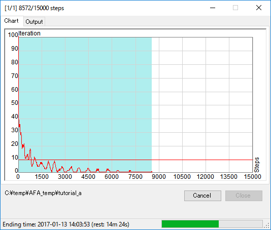
- ソルバーが起動すると下図のような「ソルバーモニター」が表示され、計算過程が表示されます。
進捗状況を示す折れ線がグラフの右端まで進めば計算完了です。
- When the solver starts up, "Solver Monitor" appears and shows the computational process.
When the line indicating the computational progress reach the right end, the computation is complete.
計算実行中
Computation in progress
計算完了
Computation completed
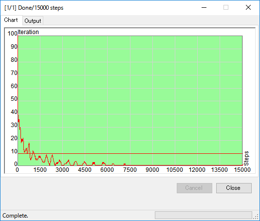
- 計算終了後は[閉じる]をクリックして、ソルバーモニターを閉じてください。
- After computation was finished, click [Close] to close Solver Monitor.
シミュレーションデータを出力する
Export simulation data
ソルバーによる計算が完了したら、結果データをまとめて、NetCDF形式のシミュレーションデータファイルに出力します。
After the solver completed computation, organize the result data and export to a simulation data file in the netCDF format.
可視化用NetCDFファイルの出力
Exporting a netCDF file for visualization
- ソルバーの計算結果は、作業ディレクトリ内の瞬間値データファイル(3d-inst-vis.dat)に格納されています。
この計算結果をArcScene上で可視化するために、解析ツールバーの
[
 Export Simulation Result (風況解析結果をNetCDF形式で出力)]をクリックします。
- The results of computation are stored as instantaneous value data (3d-inst-vis.dat) in the working directory.
To visualize them in ArcScene, click [Export Simulation Result File] on the Analysis Toolbar.
- フォルダー選択ダイアログボックスで作業ディレクトリの場所を指定すると、
[Settings to Export NetCDF File (NetCDF出力設定)]ダイアログボックスが表示されます。
- In the folder selection dialog box, select the working directory,
and then the [Settings to Export NetCDF File] dialog box appears.
- [Data Source (データソース)]タブで、NetCDFファイルに含める計算結果データを選択します。
下表のように設定してください。
- On the [Data Source] tab, select the result data to be included in the netCDF file.
Edit settings as follows.
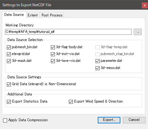
| [Data Source Selection (データソース選択)] |
オンにできるものは全部オン
All things that can be turned on
|
| [Grid Data is Non-Dimensional (無次元の格子モデル座標を使用)] |
オン
On
|
| [Export Statistics Data (統計データを出力する)] |
オン
On
|
| [Export Wind Speed & Direction (風速値と風向を出力する)] |
オン
On
|
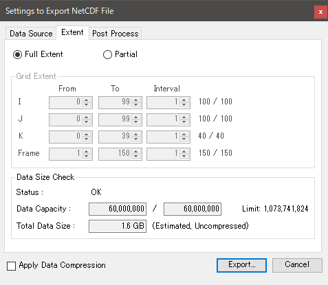
- 次に、[Extent (出力範囲)]タブをクリックし、格子とフレームの出力範囲を指定します。
ドライブの空き容量に余裕があるなら、[Full Extent (全域)]を選択します。
(本チュートリアルの通りの設定でソルバーを実行し、全域を出力した場合、ファイルサイズは約1.6GBになります。)
- Click the [Extent] tab, set the export range of the grid and the computational frame.
In this tutorial, select [Full Extent].
(If the computation is performed according to the settings as in this tutorial and the whole area is output, the file size will be about 1.6 GB.)
- [Post Process (後処理設定)]タブをクリックし、シミュレーションの風速を実際の風速スケールに換算する設定を行います。
本チュートリアルでは、流入断面付近において、地上高30.0m付近で5.0m/sの風況観測がなされた場合を想定し、
下図のように設定します。
- Click the [Post Process] tab, set parameters to convert the wind speed of the simulation to the real wind speed scale.
In this tutorial, considering a wind observation of 5.0 m/s at 30.0 m height above the ground near the inlet section,
edit settings as follows.
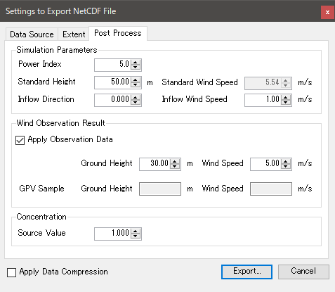
| [Apply Observation Data (観測値を適用する)] |
オン
On
|
| [Ground Height (地上高)] |
"30.00" |
| [Wind Speed (風速)] |
"5.00" |
- 各種設定後、[Export (出力)]をクリックします。
- After completing settings, click [Export].
- ファイル保存ダイアログボックスで、NetCDFファイルの出力先を指定して[Save (保存)]をクリックすると、
データ変換処理およびNetCDFファイル出力が行われます。
本チュートリアルでは、作業ディレクトリに、デフォルトの"rcdata.nc"というファイル名で保存します。
- In the save file dialog box, select the destination netCDF file, and click [Save].
Wait data conversion process, and then the netCDF file export is done.
In this tutorial, save a netCDF file with the default file name, "rcdata.nc", in the working directory.
風況シミュレーションの可視化
Visualize the wind simulation
風況シミュレーションデータファイルができたら、様々なレンダラー(描画機能)で風況などを可視化できます。
本チュートリアルでは、いくつかのレンダラーを使ってみます。
Once a wind simulation data file was created, you can visualize wind conditions and others with various renderers (drawing functions).
In this tutorial, we will try using some renderers.
新規可視化プロジェクト
New visualization project
- Airflow Analyst 可視化ツールバーの[Visualization Project (可視化プロジェクト) > New (新規)]をクリックします。
- Click [Visualization Project > New] on the Visualization Toolbar.
- ファイル選択ダイアログボックスで、前章で作成したシミュレーションデータNetCDFファイル"rcdata.nc"を選択し、[Open (開く)]をクリックします。
- In the file selection dialog box, select the simulation data netCDF file for visualization ("rcdata.nc"), and click [Open].
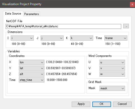
- [Visualization Project Property (可視化プロジェクトのプロパティ)]ダイアログボックスが表示されます。
デフォルト設定のまま、[OK]をクリックします。
- In the [Visualization Project Property] dialog box, leave the default settings, and click [OK].
- データの読み込みが正常に行われると、可視化ツールバーの各種機能が有効になります。
- When the data has been loaded successfully, functions for visualization will be enabled as follows.
格子可視化設定
Grid visualization settings
可視化ツールバーの[View (表示) > Grid Visualization Settings (格子可視化設定)]をクリックすると、
[Grid Visualization (可視化設定)]ダイアログボックスが表示されます。
このダイアログボックスで各種レンダラーの設定を行います。
Click [View > Grid Visualization Settings] on the Visualization Toolbar, then the [Grid Visualization] dialog box appears.
Use this dialog box to set up various renderers.
- レンダラー一覧
- List of renderers
リスト中のレンダラー名をクリックすると、設定編集タブが表示されます。
Click a renderer name in the list to show the renderer setting tab.
- レンダラー表示・非表示チェックボックス
- Renderer on / off check box
各レンダラーの表示・非表示を切り替えます。
Toggle visibility of each renderer.
格子線レンダラー
Grid Line Renderer
格子線レンダラーは、格子線を表示する描画機能です。
Grid Line Renderer draws mesh lines of the grid.
- [Grid Visualization (可視化設定)]ダイアログボックスの[Add New Renderer (新規レンダラー) > Grid Line (格子線)]をクリックすると、
格子線レンダラーが追加されます。
- Click [Add New Renderer > Grid Line] in the [Grid Visualization] dialog box to add a Grid Line Renderer.
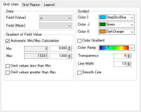
- [Grid Region (格子領域)]タブをクリックし、格子領域テーブルで各格子面の[On (表示)]を切り変えてみてください。
- Click the [Grid Region] tab, try changing the [On] of each grid section in the table.
格子マスク・レンダラー
Grid Mask Renderer
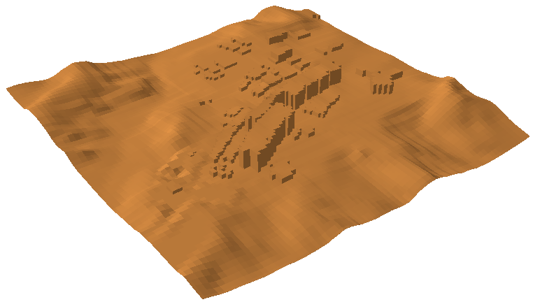
格子マスク・レンダラーは、地表面や物体の形状を表示する描画機能です。
Grid Mask Renderer draws how the geometries of the buildings and other objects are captured on the grid.
- [Grid Visualization (可視化設定)]ダイアログボックスの[Add New Renderer (新規レンダラー) > Grid Mask (格子マスク)]をクリックすると、
格子マスク・レンダラーが追加されます。
- Click [Add New Renderer > Grid Mask] in the [Grid Visualization] dialog box to add a Grid Mask Renderer.
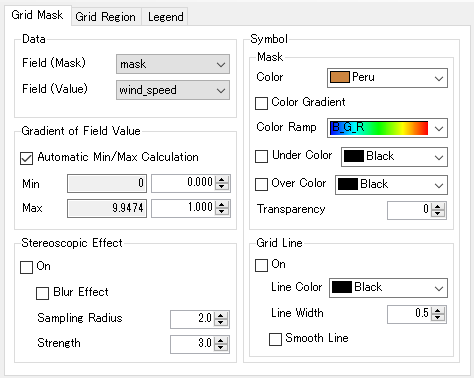
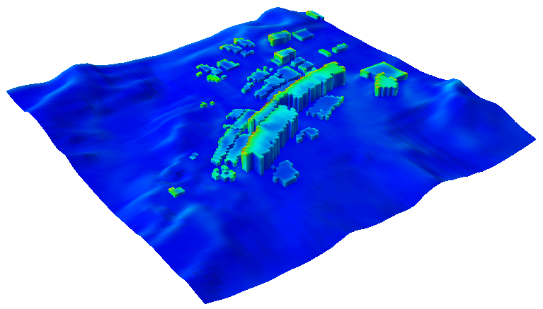
- [Grid Mask (格子マスク)]タブで、[Symbol (シンボル)]欄の[Color Gradient (フィールド値でグラデーション)]をオンにすると、
[Field (Value ) (フィールド(値))]で指定されたデータの値を色で表すことができます。
右下図は、[Field (Value) (フィールド(値))]を"avg_speed"に設定し、建物壁面の平均風速を示した例です。
- On the [Grid Mask] tab, if you select [Color Gradient] in the [Symbol] group,
the value of the data specified in [Field (Value)] can be expressed in color.
In the lower right figure, [Field (Value)] is set to "avg_speed", and the average wind speed on the wall of the building is shown.
等値線レンダラー
Contour Line Renderer
等値線レンダラーは、風速や拡散物質の濃度などの分布を、指定した断面で等値線として表現する描画機能です。
Contour Line Renderer draws contour lines on a specified section
expressing the distributions of the wind speed, concentration of diffusion materials, and other variables.
- [Grid Visualization (可視化設定)]ダイアログボックスの[Add New Renderer (新規レンダラー) > Contour Line (等値線)]をクリックすると、
等値線レンダラーが追加されます。
- Click [Add New Renderer > Contour Line] in the [Grid Visualization] dialog box to add a Contour Line Renderer.
- [Contour (等値線)]タブで、下図のように設定を変更します。
- On the [Contour] tab, edit settings as follows.
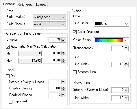
| [Field (Value) (フィールド(値))] |
"wind_speed" |
| [Color Gradient (フィールド値でグラデーション)] |
オン
On
|
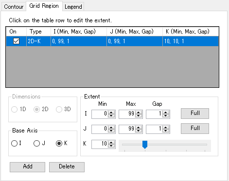
- [Grid Region (格子領域)]タブをクリックします。
[Extent (範囲)]欄で、[K]のスライダーバーを動かして値を"10"に変更すると、水平断面(K=10)の等値線が描画されます。
- Click the [Grid Region] tab.
Move the [K] slider bar to "10", and then contour lines on the horizontal section (K=10) are drawn.
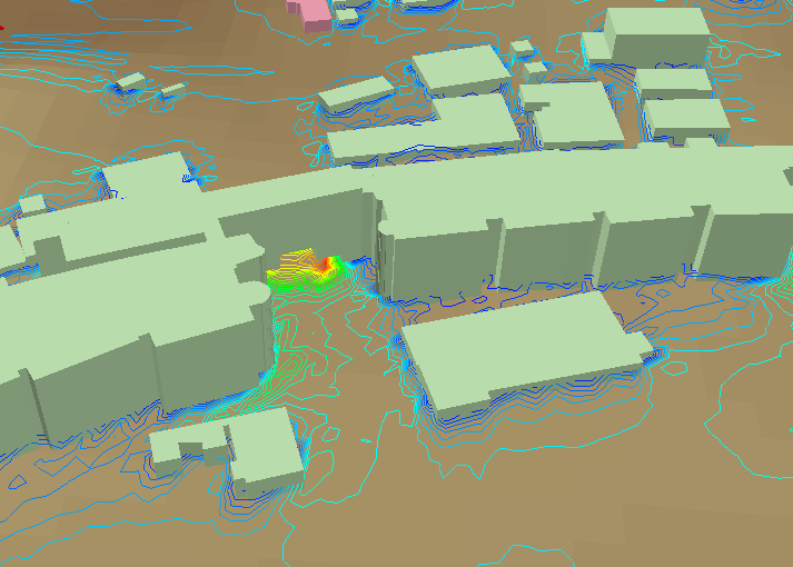
- 可視化ツールバーの[
 Start (アニメーション再生)]をクリックすると、
風速分布がアニメーション表示されます。
Start (アニメーション再生)]をクリックすると、
風速分布がアニメーション表示されます。
- When you click [Start] on the Visualization Toolbar,
the wind speed distribution is animated.
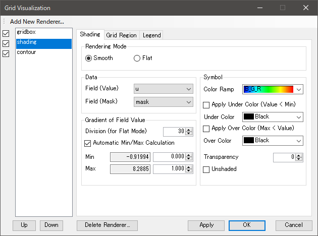
シェーディング・レンダラー
Shading Renderer
シェーディング・レンダラーは、風速や、放出された物質の濃度などの分布をグラデーション表示された面として表現する描画機能です。
以下に、地表面付近の風速分布を可視化する手順を示します。
Shading Renderer draws gradation on a specified section
expressing the distributions of the wind speed, concentration of diffusion materials, and other variables.
Here is the procedure for visualizing wind speed distribution near the ground surface.
- [Grid Visualization (可視化設定)]ダイアログボックスの[Add New Renderer (新規レンダラー) > Shading (シェーディング)]をクリックすると、
シェーディング・レンダラーが追加されます。
- Click [Add New Renderer > Shading] in the [Grid Visualization] dialog box to add a Shading Renderer
- [Shading (シェーディング)]タブで、下図のように設定を変更します。
- On the [Shading] tab, edit settings as follows.
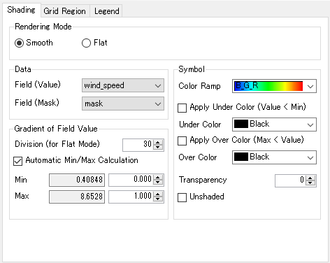
| [Rendering Mode (描画モード)] |
"Flat (フラット)" |
| [Field (Value) (フィールド(値))] |
"wind_speed" |
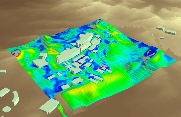
- [Grid Region (格子領域)]タブをクリックします。
[Extent (範囲)]欄で、[K]のスライダーバーを動かして値を"10"に変更すると、水平断面(K=10)の風速分布が描画されます。
- Click the [Grid Region] tab.
Move the [K] slider bar to "10", and then wind speed distribution on the horizontal section (K=10) is drawn.
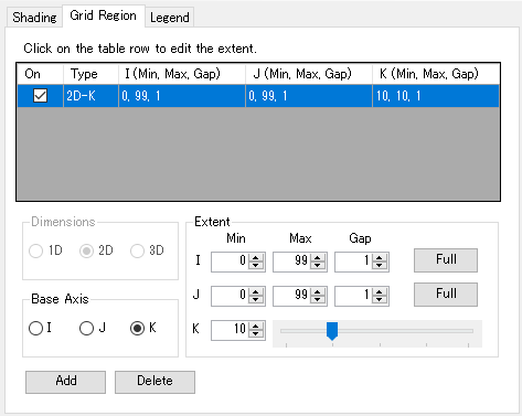
- 格子領域テーブルの[Type]="2D-K"の行の[On (表示)]をクリックしてチェックを外し、K層を非表示にします。
- Clear [On] of the row [Type]="2D-K" to hide the K-section.
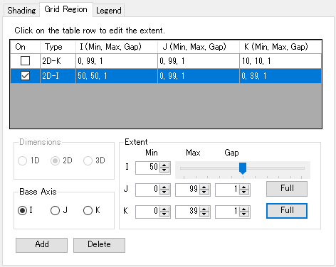
- I層の表示断面設定を追加するため、[Add (追加)]をクリックし、[Base Axis (基本軸)]で"I"を選択します。
[Extent (範囲)]欄のK層の[Full (全体)]をクリックします。
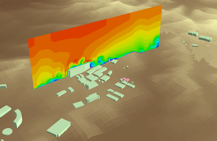
I層のスライダーバーを動かして"50"にすると、垂直断面(I=50)の風速分布が描画されます。
- To add an I-section, click [Add], and select "I" on [Base Axis].
On [Extent], click [Full] of K-section.
Move the slider bar of I-section to "50", then wind speed distribution on the vertical section (I=50) is drawn.
- 可視化ツールバーの[Start (アニメーション再生)]をクリックすると、
風速分布がアニメーション表示されます。
- When you click [Start] on the Visualization Toolbar,
the wind speed distribution is animated.
- 各種表示設定やシェーディングの表示断面位置(各断面の[層]の値)を変えながら、
どのように表現が変わるのか試してみてください。
- Try editing the renderer settings and the position of the section
to see how the expression changes.
等値面レンダラー
Contour Surface renderer
等値面レンダラーは、指定した数値の分布を立体表面として表示する描画機能です。
Contour Surface Renderer draws the distribution of a specified value as 3D surfaces.
- [Grid Visualization (可視化設定)]ダイアログボックスの[Add New Renderer (新規レンダラー) > Contour Surface (等値面)]をクリックすると、
等値面レンダラーが追加されます。
- Click [Add New Renderer > Contour Surface] in the [Grid Visualization] dialog box to add a Contour Surface Renderer.
- [Contour Surface (等値面)]タブで、下図のように設定を変更します。
- On the [Contour Surface] tab, edit settings as follows.
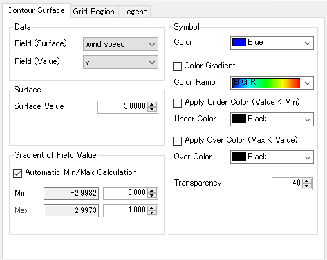
| [Field (Surface) フィールド(等値面)] |
"wind_speed" |
| [Surface Value (等値面の値)] |
"3.00" |
| [Transparency (透過度)] |
"40" |
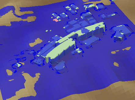
- "wind_speed=3.00"の領域が描画されます。
青い面がかかっている箇所は風速3.0m/s未満の領域であり、
建物が見えている箇所は3.0m/s以上の領域となります。
- Contour surface of "wind_speed=3.00" are drawn as the following image.
The areas covered by blue surfaces are the regions with wind speed less than 3.0 m/s,
and the areas where the buildings are visible are the regions of 3.0 m/s or more.
ベクトル・レンダラー
Vector Renderer
ベクトル・レンダラーは、格子接点上の風向や風速を3Dの矢印(風ベクトル)として表現する描画機能です。
以下に、地表面付近の風ベクトルを表示する手順を示します。
Vector Renderer draws the wind direction and the wind speed on the grid point as 3D arrows (wind vectors).
Here is the procedure for displaying the wind vector near the ground surface.
- [Grid Visualization (可視化設定)]ダイアログボックスの[Add New Renderer (新規レンダラー) > Vector (ベクトル)]をクリックすると、
ベクトル・レンダラーが追加されます。
- Click [Add New Renderer > Vector] in the [Grid Visualization] dialog box to add a Vector Renderer.
- [Vector (ベクトル)]タブで、下図のように設定を変更します。
- On the [Vector] tab, edit settings as follows.
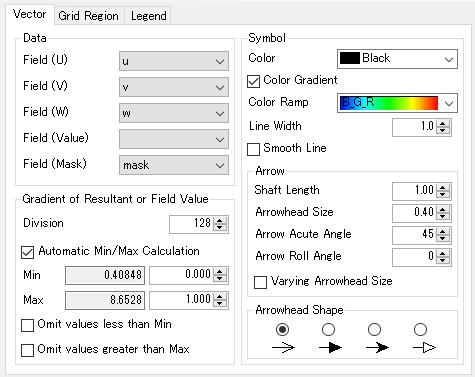
| [Field (Value) (フィールド(値))] |
空欄、または"wind_speed"を選択
leave blank or select "wind_speed"
|
| [Color Gradient (フィールド値でグラデーション)] |
オン
On
|
| [Arrowhead Size (矢先のサイズ)] |
"1.50" |
- ベクトル・レンダラーでは、[Field (Value) (フィールド(値))]を空欄にすると、
風速成分u,v,wを動的に合成してwind_speedと同じ値になります。
- As for the Vector Renderer, if you leave [Field (Value)] blank,
the wind components u, v, and w are dynamically calculated to the same value as "wind_speed".
- [Grid Region (格子領域)]タブをクリックします。
[Extent (範囲)]欄で、[K]のスライダーバーを動かして値を"10"に変更すると、水平断面(K=10)の風速・風向を表す矢印が描画されます。
- Click the [Grid Region] tab.
Move the [K] slider bar to "10", and then wind vectors on the horizontal section (K=10) are drawn.

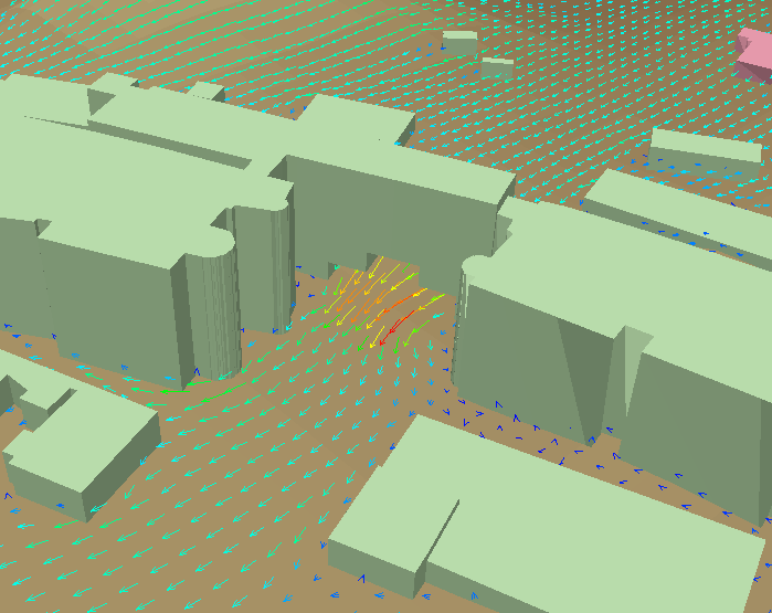
- 可視化ツールバーの[Start (アニメーション再生)]をクリックすると、
風速・風向を表す矢印がアニメーション表示されます。
- When you click [Start] on the Visualization Toolbar,
the wind vectors are animated.
- 各種表示設定やベクトルの表示断面を変えながら、
どのように表現が変わるのか試してみてください。
- Try editing the renderer settings and the position of the section
to see how the expression changes.
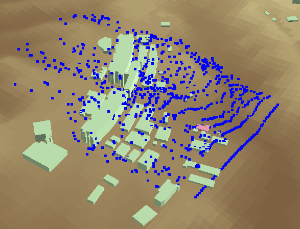
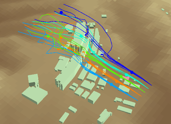
粒子追跡レンダラー
Particle Trace Renderer
粒子追跡レンダラーは、計算格子の任意の点から仮想の粒子を飛ばした場合の粒子の軌跡を表示する描画機能です。
Particle Trace Renderer displays the trajectories of virtual particles that are released from arbitrary points in the computational grid.
- [Grid Visualization (可視化設定)]ダイアログボックスの[Add New Renderer (新規レンダラー) > Particle Trace (粒子追跡)]をクリックすると、
粒子追跡レンダラーが追加されます。
- Click [Add New Renderer > Particle Trace] in the [Grid Visualization] dialog box to add a Particle Trace Renderer.
- [Particle Trace (粒子追跡)]タブで、下図のように設定を変更します。
- On the [Particle Trace] tab, edit settings as follows.
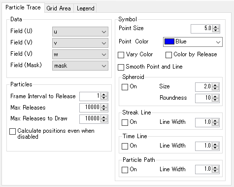
| [Frame Interval to Release (放出フレーム間隔)] |
"1" |
- [Grid Region (格子領域)]タブをクリックします。
表示断面設定を、下図のように修正します。
- Click the [Grid Region] tab.
Edit settings of the section as follows.
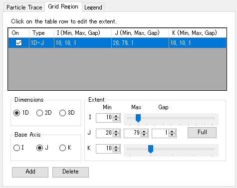
| [Dimensions (次元)] |
"1D" |
| [Base Axis (基本軸)] |
"J" |
| [I] |
"10" |
| [J_Min)] |
"20" |
| [J_Max)] |
"79" |
| [J_Gap (J (間隔))] |
"1" |
| [K] |
"10" |
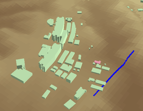
- 可視化ツールバーの[Start (アニメーション再生)]をクリックすると、
仮想粒子の移動アニメーションが表示されます。
- When you click [Start] on the Visualization Toolbar,
virtual particles start moving.
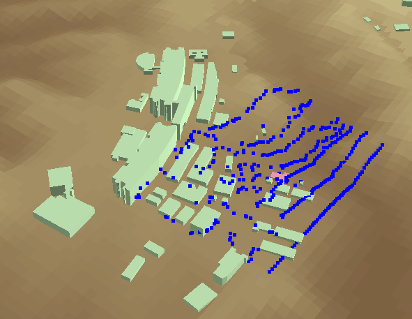
- 各種表示設定や放出位置を変えながら、どのように表現が変わるのか試してみてください。
- Try editing the renderer settings and the release positions,
to see how the expression changes.
この文書の内容は開発中のものです。
リリース時には変更となる場合があります。
The contents in this document are under development.
It may be changed at the time of release.
Copyright (C) 2018 Environmental GIS Laboratory Co.,Ltd. All rights reserved.