Airflow Analystの風況解析ソルバー「RC-GIS」の理論的背景について解説します。
We will explain the theoretical background of the wind analysis solver "RC-GIS" of Airflow Analyst.
| 計算コード Calculation code | 市街地版RIAM-COMPACT (RC-GIS) RIAM-COMPACT (RC-GIS) for City |
| 乱流モデル Turbulence model | LES LES |
| 解析手法 Analysis method | 非定常解析 Transient analysis |
| 離散化手法 Discretization method | 差分法 Difference method |
| スキーム Scheme | 補間法 Interpolation method |
| 流入境界条件 Inlet boundary condition | べき法則または気象モデルからの内挿補間により作成 Created by interpolation from power law or weather model |
| 流出境界条件 Outlet boundary condition | 対流型流出条件 Convection flow condition |
| 側面境界条件 Side boundary condition | 滑り条件 Free-slip condition |
| 上部境界条件 Upper boundary condition | 滑り条件 Free-slip condition |
| 地表面境界 Ground surface boundary | 粘着条件 No-slip condition |
| 建物側壁境界 Building side wall boundary | 粘着条件 No-slip condition |
| 収束判定 Convergence determination | RMS誤差=1.0E-3、あるいは最大反復回数100回 RMS error = 1.0E-3, or maximum iteration number 100 |
| 抵抗体モデル Resistivity model | 外力項として考慮 Consider as external force term |
RC-GISは、非圧縮性流体の連続の式とNavier-Stokes方程式に基づき、 都市域や複雑地形上の非定常な風況場をLES(Large-Eddy Simulation)により 数値シミュレーションするCFD(Computational Fluid Dynamics)ソフトウェアである。 LESでは流れ場に空間フィルターを施し、 大小様々なスケールの乱流渦を計算格子よりも大きなGS(Grid Scale)成分の渦と、 それよりも小さなSGS(Sub-Grid Scale)成分の渦に分離する。 GS成分の大規模渦は、モデルに頼らず直接数値シミュレーションを行う。 一方、SGS成分の小規模渦が担う、主としてエネルギー消散作用はSGS応力を物理的考察に基づいてモデル化する。 差分法では空間フィルターと微分操作の互換性が成立するので、 フィルター関数を陽に与える必要はない。 SGSモデルには計算安定性に優れた標準Smagorinskyモデルを採用する。 これは、局所平衡と渦粘性を仮定しており、エネルギー散逸の総量には妥当なモデルである。
RC-GIS is a CFD (Computational Fluid Dynamics) software that numerically simulates unsteady wind situations on urban areas or complex terrains by LES (Large-Eddy Simulation) based on the continuity equation of incompressible fluid and Navier-Stokes equations. In LES, a spatial filter is applied to the flow field, and turbulent eddies of various sizes are separated into eddies of the GS (Grid Scale) component larger than the computational grid and eddies of the SGS (Sub-Grid Scale) component smaller than that. Large-scale eddies of the GS component are directly subjected to numerical simulation without relying on models. On the other hand, the energy dissipation effect mainly by the small scale eddies of the SGS component models SGS stress based on physical consideration. Since the compatibility between the spatial filter and the differential operation is established by the difference method, it is not necessary to explicitly give the filter function. For the SGS model, adopt the standard Smagorinsky model with excellent computational stability. This assumes local equilibrium and eddy viscosity, and it is a reasonable model for the total energy dissipation.
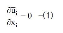
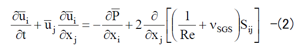
空間フィルターを施して粗視化した連続の式とNavier-Stokes方程式を以下の(1)、(2)式に示す。 但し、座標系は xi(x1=x, x2=y, x3=z) とし、 これに対応する物理速度のGS成分は ui(u1=u, u2=v, u3=w) とする。 ここで、添え字1, 2, 3は主流方向、主流直交方向、鉛直方向を示す。 速度は境界層上空の風速U、 長さは建物あるいは地形の特徴的な高さスケールH、 時間はH/U、 圧力は参照密度ρとUの積ρU2で無次元化されている。 なお、重複する添え字には総和規約が適用される。
The continuous equations and the Navier-Stokes equations which are coarse-grained by applying a spatial filter are shown in the following equations (1) and (2). The coordinate system is xi(x1=x, x2=y, x3=z), and the corresponding GS component of the physical velocity is ui(u1=u, u2=v, u3=w). Here, the suffixes 1, 2, 3 indicate the main flow direction, the main flow perpendicular direction, and the vertical direction. The velocity is dimensionless by the wind velocity U over the boundary layer, the length by the standard height scale H of the buildings or the terrain, the time by H / U, and the pressure by the product ρU2 of the reference density ρ and U. The summation convention is applied to duplicated subscripts.
(2)式中のPは総圧力と呼ばれ、以下のように定義される。
P in the equation (2) is called total pressure, and is defined as follows.

(3)式中のpは圧力のGS成分であり、 kSGSはSGS運動エネルギーで以下のように定義される。
p in the equation (3) is a GS component of the pressure, and kSGS is the SGS kinetic energy defined as follows.

(2)式中のSGS渦粘性係数νSGSは、 標準Smagorinskyモデルにおける唯一の無次元パラメーターであるSmagorinsky定数CSと 歪速度テンソルSijを用いて以下のように定義される。
The SGS eddy viscosity coefficient νSGS in the equation (2) is defined as follows using the Smagorinsky constant CS which is the only dimensionless parameter in the standard Smagorinsky model, and the strain rate tensor Sij.


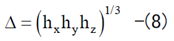
標準Smagorinskyモデルでは、 大小様々なスケールの乱流渦を分離するフィルター幅が代表長さスケールとなる。 デカルト座標系では、フィルター幅は格子幅と同じとし、各方向の格子幅 hi(=hx, hy, hz) を用いて以下のように定義される。
In the standard Smagorinsky model, the filter width separating the turbulent eddies of various sizes becomes the standard length scale. In the Cartesian coordinate system, the filter width is assumed to be the same as the grid width, and is defined as follows using the grid width hi(=hx, hy, hz) in each direction.
以上、(1)-(8)式がデカルト座標系(物理面)での標準Smagorinskyモデルに基づいたLES基礎式である。
The above equations (1) - (8) are the LES basic equations based on the standard Smagorinsky model in the Cartesian coordinate system (physical plane).
本プログラムでは、z*座標系(terrain-following vertical coordinate system)のコロケート格子に基づいた差分法により数値解を求める。 よって、上記のLES基礎式は物理面から計算面に写像される。 コロケート格子とは、計算格子のセル中心に物理速度成分と圧力を定義し、 セル界面にヤコビアンを乗じた反変速度成分を定義する格子系である。
In this program, the numerical solutions are obtained by the difference method based on the collocated grid of the z* coordinate system (terrain-following vertical coordinate system). Therefore, the above LES basic equations are mapped from the physical plane to the calculation plane. A collocated grid is a grid system that defines physical velocity components and a pressure at the cell center of a computational grid, and defines anti-shift components by multiplying Jacobian at the cell interfaces.
速度場と圧力場のカップリングアルゴリズムには、 Eulerの一次陽解法を基礎とした部分段階法を採用する。 圧力は、2段階に分けた(2)式のうち圧力勾配項を含む式を(1)式に代入してPoisson方程式を導き、 SOR法(Successive Over Relaxation method)により緩和計算して算出する。 空間項の離散化に関して、(2)式の対流項には、補間法による4次精度中心差分に4階微分の数値粘性項を付加した3次精度風上差分を用いる。 ここで、数値粘性項の重みはα=0.5とし、その影響は十分に小さくしている。 一般に使用される3次精度風上差分のKawamura-Kuwaharaスキームでは、α=3である。 残りの全ての空間項には、2次精度中心差分を適用した。 実際の計算手順は以下に示すとおりである。
For the coupling algorithm between the velocity field and the pressure field, the partial step method based on Euler's first explicit method is adopted. To calculate the pressure, substitute an expression including the pressure gradient term in the equation (2) divided into two stages into the equation (1) to derive the Poisson equation, and perform relaxation calculation by the SOR (Successive Over Relaxation) method. Regarding the discretization of the spatial term, for the convection term of equation (2), we use the third-order upwind difference obtained by adding the numerical viscosity term of the fourth-order derivative to the fourth-order central difference by the interpolation method. Here, the weight of the numerical viscosity term is set to α = 0.5, and its influence is sufficiently small. In the Kawamura-Kuwahara scheme commonly used as a third-order upwind difference, α = 3. Second-order central difference was applied to all remaining spatial terms. The actual calculation procedure is as follows.