Airflow Analystアドイン クイックスタートチュートリアル

Airflow Analyst Add-In Quick Start Tutorial

本チュートリアルでは、計算格子の作成から気流解析ソルバーの実行、解析データの可視化まで、 Airflow Analystアドインによる風況シミュレーションの手順を案内します。

In this tutorial, we will guide you through the procedure of wind simulation with the Airflow Analyst add-in from creating a computational grid to executing an airflow analysis solver, and visualizing analysis data.

チュートリアルの準備

Prepare for the tutorial

Airflow Analystアドインのセットアップ

Set up Airflow Analyst add-in

セットアップガイドを参考に、Airflow Analystアドインを利用可能な状態にします。

Make the Airflow Analyst add-in available by referring to the Setup Guide.

チュートリアル用ArcGIS Proプロジェクト

ArcGIS Pro project for the tutorial

1. Airflow Analystアドインのチュートリアル用データをダウンロードします。
2. Download tutorial data of the Airflow Analyst add-in.
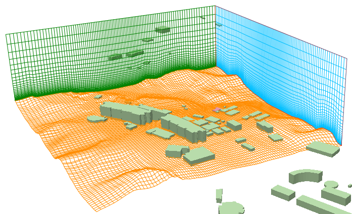
3. ダウンロードしたファイルを展開し、 チュートリアル用ArcGIS ProマップファイルTutorial.mapxを開きます。 ArcGIS Proが起動し、地形と建物が3Dで表示されます。
4. Unzip the downloaded file, and open an ArcGIS Pro map file for the tutorial Tutorial.mapx. ArcGIS Pro will startup, and then the terrain and buildings will be displayed in 3D.
5. ArcGIS Proのリボンに Airflow Analyst - 解析タブとAirflow Analyst - 可視化タブが 追加されているか確認してください。
6. Make sure that the Airflow Analyst - Analysis and Airflow Analyst - Visualization tabs have been added to the ArcGIS Pro ribbon.

計算格子の作成

Create a computational grid

まず、シミュレーション範囲の計算格子を作成します。

First, create a computational grid for the simulation area.

新規解析プロジェクト

New analysis project

1. リボンのAirflow Analyst - 解析タブを開き、 解析プロジェクトグループの[新規]をクリックします。
   シーンの中央に格子が表示されます。
2. On the ribbon, go to the Airflow Analyst - Analysis tab. In the Analysis Project group, click [New].
   A grid appears in the center of the scene.

計算格子の設定

Settings of a computational grid

1. リボンの解析タブの格子グループにある [格子位置]ツールをクリックします。
2. On the Analysis tab on the ribbon, in the Grid group, click the [Grid Position] tool.
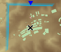
3. ローカルシーン上で、計算領域の基準点となる位置をクリックします。 本チュートリアルでは、下図の×印で指したあたりをクリックします。 別の場所をクリックすれば、基準点を修正できます。
   何もない空間をクリックしても位置取得できないので、地形か建物の上をクリックしてください。
4. On the local scene, click at a location to make the reference point of the analysis area. In this tutorial, click on X in the following figure. You can modify the point by clicking at a different location.
   If you click at a space with nothing, you cannot get the coordinates, so click on the terrain or buildings.



5. マップに計算格子が描画され、計算格子設定ダイアログボックスが表示されます。
6. A computational grid is drawn on the map, and the Grid Settings dialog box will open.
• 位置タブで、格子の位置や向きを設定します。
• On the Location tab, set the position of the grid.

経度 Longitude	(クリック位置) (Clicked position)
緯度 Latitude	(クリック位置) (Clicked position)
標高 Altitude	(クリック位置) (Clicked position)
流入風向 Inflow direction	0.0 (北) 0.0 (North)
地表面標高レイヤー Terrain elevation layer	Elevation.tif
地表面の格子を滑らかに Smooth terrain elevation	On

• サイズ(水平方向)タブで、格子の水平方向のサイズを設定します。
• On the Size (Horizontal) tab, set the horizontal size of the grid.

	値 (I) Value (I)	値 (J) Value (J)
水平方向 格子生成 Horizontal gridding	単焦点 Single Focus
格子点数 Number of nodes	100	100
基本格子間隔 Default node spacing	5.00	5.00
基本間隔格子点数 Number of default spacing nodes	10	10
格子間隔増加率 Stretch ratio	1.020	1.020
偏心格子オフセット Focus offset	0	0

• サイズ(鉛直方向)タブで、格子の水平方向のサイズを設定します。
• On the Size (Vertical) tab, set the vertical size of the grid.

鉛直方向 格子生成 Vertical gridding	頂部平面 Flat Top
代表高さ Standard height	50.00
高さ補正係数 Height correction factor	5
格子点数 Number of nodes	40

• 属性タブで、格子内部の物体を設定します。
• On the Attributes tab, set objects inside the grid.
1. 物体レイヤー欄の[追加]をクリックします。
2. In the Object layers group, click [Add].
3. 物体レイヤー設定ダイアログボックスで、 下記のように設定し、[OK]をクリックします。
4. In the Object Layer Settings dialog box, edit the settings as follows, and click [OK].

物体レイヤー Object layer	Building
物体判定方法 Object scan method	K層揃え Along K
地面の標高 Ground elevation	ELEVATION
物体の高さ Object height	HEIGHT
地面からのオフセット Offset from the ground	OFFSET
物体種別コード Object type code	FLAG

5. 前項の設定により、物体レイヤーテーブルに"Building"レイヤーが追加されます。
   設定を修正する場合は、対象となる行を選択して[編集]をクリックするか、行をダブルクリックしてください。
6. By the setting in the previous section, a "Building" layer is added to the object layers table. To correct the setting, select the row and click [Edit], or double-click the row.
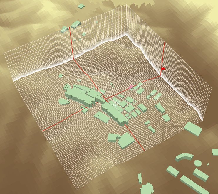
7. ダイアログボックスの[OK]をクリックして、格子設定を確定します。 シーン上に下図のような格子が表示されます。
8. Click [OK] in the dialog box to confirm the grid settings. A grid is generated as follows.



9. 格子設定を修正する際は、 リボンの解析タブの格子グループにある [格子設定]をクリックすると、 計算格子設定ダイアログボックスが表示されます。
10. If you want to modify the grid settings, on the Analysis tab on the ribbon, in the Grid group, click [Grid Settings] to show the Grid Settings dialog box.

以上で、シミュレーションに必要な計算格子設定は完了です。

Setting up the computational grid for the simulation is completed.

解析プロジェクトの保存

Save an analysis project

1. ディスク容量に余裕があり、高速にアクセスできるドライブに任意の名前のフォルダーを作成します。
2. Create a folder of any name on a drive that has sufficient capacity and fast access.
3. リボンの解析タブの解析プロジェクトグループにある [保存]をクリックします。
4. On the Analysis tab on the ribbon, in the Analysis Project group, click [Save].
5. ファイル保存ダイアログボックスで、 先ほど作成したフォルダーに移動し、解析プロジェクトファイル "project.aaa" を保存します。
   (このファイルが存在するフォルダーが、解析データを保管する作業ディレクトリとなります。)
6. In the save file dialog box, move into the working directory previously created, and save an Analysis Project file "project.aaa".
   (The folder where this file exists is the Working Directory for storing analysis data.)

気流解析ソルバー「RC-GIS」の実行

Run an airflow analysis solver "RC-GIS"

解析設定データファイルを作成し、気流解析ソルバー「RC-GIS」を実行します。

Create analysis setting data files, and then run an airflow analysis solver "RC-GIS".

解析設定

Analysis settings

1. リボンの解析タブの気流解析グループにある [解析設定]をクリックします。
2. On the Analysis tab on the ribbon, in the Airflow Analysis group, click [Analysis Settings].
3. 気流解析設定ダイアログボックスで、解析設定を編集します。 (下表は大気安定度対応ソルバーの場合です。)
4. In the Airflow Analysis Settings dialog box, edit solver settings. (The following table shows the case of the solver corresponding to atmospheric stability.)

べき指数 Power index	5.0
無次元時間刻み Non-dimensional tick	0.0020
計算モード Mode	気流場 Flow
リチャードソン数 Richardson number	0.0
透過度 Permeability	1.5

解析設定データファイルの出力・ソルバー実行

Output analysis setting data files, and run a solver

1. リボンの解析タブの気流解析グループにある [解析準備・実行]をクリックします。
2. On the Analysis tab on the ribbon, in the Airflow Analysis group, click [Prepare / Run Analysis].
3. 気流解析準備・実行ダイアログボックスで、 ソルバーの実行オプションを編集します。
4. In the Prepare / Run Airflow Analysis dialog box, edit the solver runtime options.

このチュートリアルでは、計算を短時間で終わらせるため、ステップ数を少なめに設定しています。

In this tutorial, the number of steps is set to a small number to finish the computation in a short time.

計算モード Computation mode	新規 New
総ステップ数 Total steps	2000
記録間隔 Recording interval	50
統計開始ステップ Start statistics from	自動 Auto
解析ケース Analysis cases	シングル Single

5. [1. 解析設定データ作成]をクリックします。
   解析に必要な設定データファイルが作業ディレクトリに出力されます。
6. Click [1. Create Analysis Setting Data Files].
   A set of setting data files for the analysis will be created in the working directory.
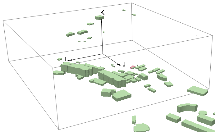
7. [2. 格子データ確認]をクリックします。
   上記で作成されたデータが読み込まれ、格子線と物体格子点がシーン上に表示されます。 格子データ表示ダイアログボックスを閉じると、格子も消えます。
8. Click [2. Check Grid Data].
   The data created above is read in and the grid lines and object grid points are displayed on the scene. Closing the Display Grid Data dialog box also clears the grid.
9. [3. ソルバー実行]をクリックします。
   風況解析ソルバー「RC-GIS」が起動します。
10. Click [3. Run Solver].
    An airflow analysis solver "RC-GIS" is to be started.
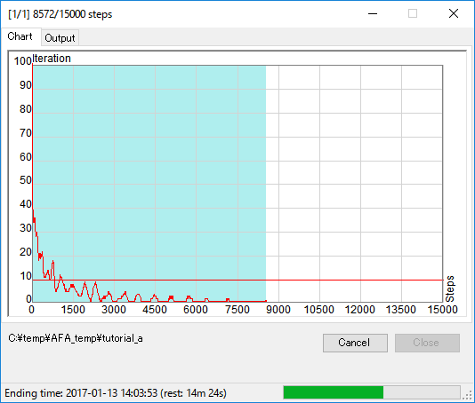
11. ソルバー進捗グラフ画面が表示され、計算過程を確認できます。 進捗状況を示す折れ線がグラフの右端まで進めば計算完了です。
12. The solver progress chart window appears, and you can check the process of the computation. When the line indicating the progress reaches the right end, the computation is complete.

計算実行中 Computation in progress


13. RC-GISは、全格子点における時系列値(風速成分、圧力、濃度)と、 時間平均値(風速成分)を出力します。 これらの解析結果データは作業ディレクトリに保存されます。
14. The solver outputs time-series values (wind speed components, pressure, concentration) and time-averaged values (wind speed components) of all grid points. These analysis result data are saved in the working directory.
15. 計算終了後は、ソルバー進捗グラフ画面の[閉じる]をクリックしください。
16. After computation was finished, click [Close] on the solver progress chart window.

シミュレーションデータファイルの作成

Create a simulation data file

ソルバーによる計算が完了したら、可視化や外部利用のため、 一連の解析データ(解析設定や結果データなどの.datファイル群)をまとめてNetCDF形式のシミュレーションデータファイルに出力します。

After the solver computation is complete, aggregate a set of analysis data (.dat files as analysis settings and result data) into a netCDF format simulation data file for visualization and external use.

後処理設定

Post processing

1. リボンの解析タブの後処理グループにある [後処理設定]をクリックすると、 後処理設定ダイアログボックスが表示されます。
2. On the Analysis tab on the ribbon, in the Post Processing group, click [Post-Process Settings] to open the Post-Process Settings dialog box.
3. パラメータタブで、下記のように設定します。
   本チュートリアルでは、流入断面付近において、地上高30.0m付近で5.0m/sの風況観測がなされた場合を想定しています。
4. On the Parameters tab, edit the settings as follows.
   In this tutorial, it is assumed that a wind condition of 5.0 m/s is observed near the inlet section at 30.0 m height above the ground.

観測値を適用する Apply observation data	On
観測値 : 地上高 Observation : Ground height	30.00
観測値 : 風速 Observation : Wind speed	5.00

5. 各種設定後、[OK]をクリックします。
6. After completing the settings, click [OK].

シミュレーションデータファイルの出力

Export a simulation data file

1. リボンの解析タブの後処理グループにある [解析データ変換]のアイコンをクリックすると、 解析データ変換ダイアログボックスが表示されます。
2. On the Analysis tab on the ribbon, in the Post Processing group, click [Convert Analysis Data] icon to open the Convert Analysis Data dialog box.
3. データソースタブで、下表のように設定します。
4. On the Data Source tab, edit the settings as follows.

格子データ	全部On On all
ソルバー結果データ	全部On On all
ソルバー結果データの計算と統計	全部On On all

5. 各種設定後、[エクスポート]をクリックします。
6. After completing the settings, click [Export].
7. ファイル保存ダイアログボックスで、NetCDFファイルの出力先を指定して[保存]をクリックします。
   出力先は、作業ディレクトリ以外でもかまいません。 本チュートリアルでは、デフォルトの"rcdata.nc"というファイル名で保存します。
8. In the save file dialog box, select a destination netCDF file, and click [Save].
   The export destination can be anything other than the working directory. In this tutorial, save a netCDF file with the default file name "rcdata.nc".

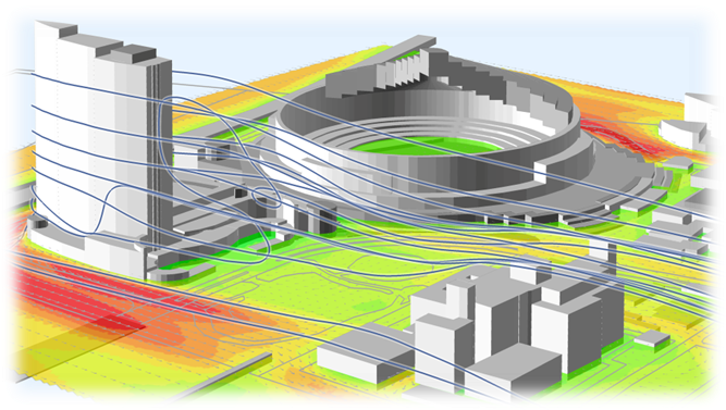
風況シミュレーションの可視化

Visualize a wind simulation

格子の形状や風速分布などを、様々なレンダラー(描画機能)でローカルシーンに表示できます。

The airflow analysis data can be visualized with various renderers (drawing functions).

新規可視化プロジェクト

New visualization project

1. リボンのAirflow Analyst - 可視化タブを開き、 可視化プロジェクトグループの[新規](.nc)をクリックします。
2. On the ribbon, go to the Airflow Analyst - Visualization tab. In the Visualization Project group, click [New (.nc)].
3. ファイル選択ダイアログボックスで、 前章で作成したシミュレーションデータファイル"rcdata.nc"を選択し、 [開く]をクリックします。
4. In the file selection dialog box, select the simulation data file "rcdata.nc" created in the previous section, and click [Open].
5. 可視化プロジェクトのプロパティダイアログボックスが表示されます。 そのまま、[OK]をクリックします。
6. The Visualization Project Properties dialog box is displayed. Just click [OK].
7. データの読み込みが正常に行われると、可視化タブの各種コマンドが有効になります。
8. When the data has been loaded successfully, commands on the Visualization tab will be available.

[レンダラー設定]ダイアログボックスの表示

Open the [Renderers] dialog box

リボンの可視化タブのレンダリンググループの [レンダラー]をクリックすると、 レンダラー設定ダイアログボックスが表示されます。

On the Visualization tab on the ribbon, in the Rendering group, click [Renderers] to open the Renderers dialog box.

• [新規レンダラー]メニュー
• [Add New Renderer] menu

各種レンダラーを追加できます。 主なレンダラーについて下記で紹介します。

You can add various renderers. Some major renderers are introduced below.

• レンダラー一覧
• List of renderers

レンダラー一覧でレンダラー名をクリックすると、設定フォームが表示されます。

Click a renderer name in the list to show each renderer setting form.

チェックボックスで、各レンダラーの表示・非表示を切り替えます。

Turn on or off the checkbox to show or hide each renderer.

格子枠レンダラー

Grid box renderer

格子枠レンダラーは、格子の外枠を描画します。 可視化プロジェクト作成時に、最初から追加されています。

The grid box renderer draws the outer lines of a grid. It is added when a visualization project is created.

[新規レンダラー]メニューの [格子枠]をクリックして追加します。

On the [Add New Renderer] menu, click [Grid Box] to add this renderer.

格子線レンダラー

Grid line renderer

格子線レンダラーは、格子線を描画します。

The grid line renderer draws mesh lines of a grid.

[新規レンダラー]メニューの [格子線]をクリックして追加します。

On the [Add New Renderer] menu, click [Grid Line] to add this renderer.

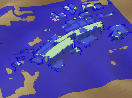
格子マスク レンダラー

Grid mask renderer

格子マスク レンダラーは、格子内の物体の形状を描画します。

The grid mask renderer draws the shape of objects in a grid.

[新規レンダラー]メニューの [格子マスク]をクリックして追加します。

On the [Add New Renderer] menu, click [Grid Mask] to add this renderer.

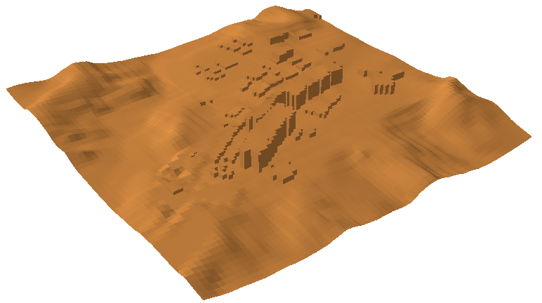
• 格子マスクの表面の圧力値をグラデーション表示する場合 :
• Display the pressure value on the surface of the grid mask in gradation :
1. 格子マスクタブで、下記のように設定します。
2. On the Grid Mask tab, edit the settings as follows.

フィールド(値) Field (Value)	pressure
表面における値	外側
グラデーション Gradient	On

等値線レンダラー

Contour line renderer

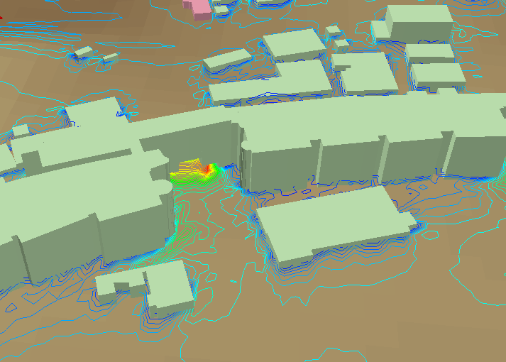
等値線レンダラーは、 指定した断面における風速や濃度などの分布を等値線で描画します。

The contour line renderer draws contour lines on a specified section expressing the distributions of the wind speed, the concentration of diffusion materials, and other variables.

[新規レンダラー]メニューの [等値線]をクリックして追加します。

On the [Add New Renderer] menu, click [Contour Line] to add this renderer.

• 水平断面 K=10における風速分布を等値線で表示する場合 :
• Display wind speed distribution on the horizontal section (K=10) with contour lines :
1. 等値線タブで、下記のように設定を変更します。
2. On the Contour tab, edit the settings as follows.

フィールド(値) Field (Value)	wind_speed
グラデーション Gradient	On

3. 格子領域タブで、[K]を"10"に設定します。
4. On the Grid Region tab, set [K] to "10"

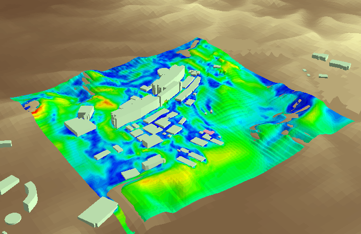
シェーディング レンダラー

Shading renderer

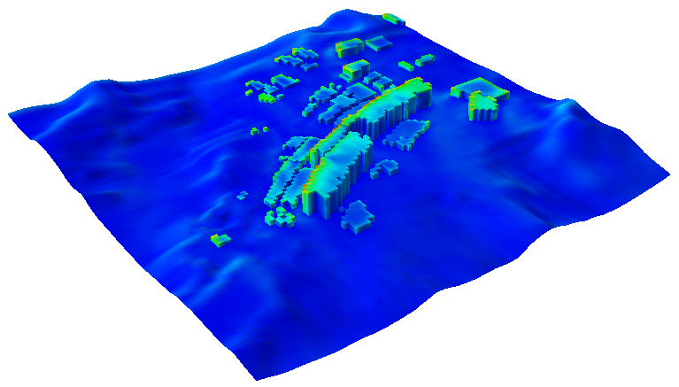
シェーディング レンダラーは、 指定した断面における風速や濃度などの分布をグラデーション表示します。

The shading renderer draws gradation on a specified section expressing the distributions of the wind speed, the concentration of diffusion materials, and other variables.

[新規レンダラー]メニューの [シェーディング]をクリックして追加します。

On the [Add New Renderer] menu, click [Shading] to add this renderer.

• 水平断面 K=10における風速分布をグラデーション表示する場合 :
• Display wind speed distribution on the horizontal section (K=10) with gradation :
1. シェーディングタブで、下記のように設定を変更します。
2. On the Shading tab, edit the settings as follows.

フィールド(値) Field (Value)

wind_speed

3. 格子領域タブで、[K]を"10"に設定します。
4. On the Grid Region tab, set [K] to "10".

等値面レンダラー

Contour surface renderer

等値面レンダラーは、指定した値の分布を3Dの面として描画します。

The contour surface renderer draws the distribution of a specified value as 3D surfaces.

[新規レンダラー]メニューの [等値面]をクリックして追加します。

On the [Add New Renderer] menu, click [Contour Surface] to add this renderer.

• 風速値が3.0の領域を表示する場合 :
• Display the area where the wind speed value is 3.0 :
1. 等値面タブで、下記のように設定を変更します。
2. On the Contour Surface tab, edit the settings as follows.

フィールド(等値面) Field (Surface)	wind_speed
等値面の値 Surface value	3.00
透過度 Transparency	40

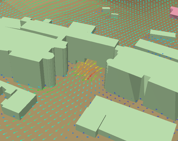
ベクトル レンダラー

Vector renderer

ベクトル レンダラーは、各格子点における風ベクトル(風向や風速を示す矢印)を描画します。

The vector renderer draws wind vectors (arrows indicating the direction and speed of the wind) on each grid point.

[新規レンダラー]メニューの [ベクトル]をクリックして追加します。

On the [Add New Renderer] menu, click [Vector] to add this renderer.

• 水平断面 K=10における風ベクトルを表示する場合 :
• Display wind vectors on the horizontal section (K=10) :
1. 格子領域タブで、[K]を"10"に設定します。
2. On the Grid Region tab, set [K] to "10".

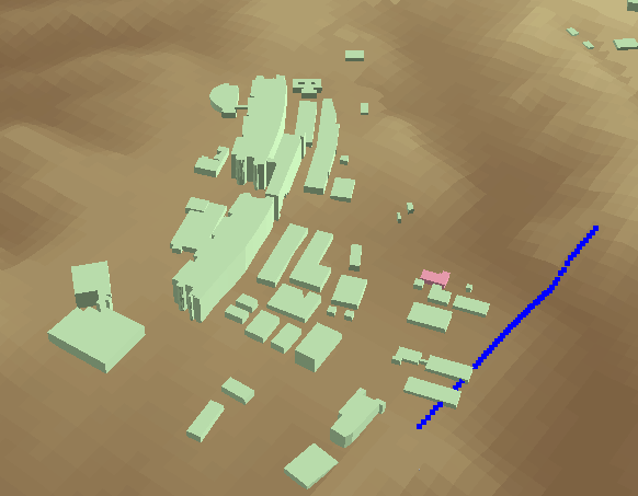
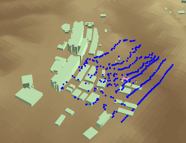
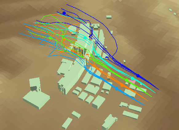
粒子追跡レンダラー

Particle trace renderer

粒子追跡レンダラーは、任意の格子点から仮想の粒子を飛ばした軌跡を計算して描画します。

The particle trace renderer displays the trajectories of virtual particles that are released from arbitrary points in the computational grid.

[新規レンダラー]メニューの [粒子追跡]をクリックして追加します。

On the [Add New Renderer] menu, click [Particle Trace] to add this renderer.

• リボンの可視化タブのフレームアニメーショングループにある [開始]をクリックすると、 仮想粒子の移動アニメーションが表示されます。
• On the Visualization tab on the ribbon, in the Frame Animation group, click [Start] to start moving the virtual particles.

• 粒子を10フレーム毎に放出し、その軌跡を表示する場合 :
• Display trace lines of particles released every 10 frames :
1. 粒子追跡タブで、下表のように設定します。
2. On the Particle Trace tab, edit the settings as follows.

流跡線 Particle path lines	On
放出フレーム間隔 Frame interval to release	10
グラデーション Gradient	On
離散的 Discrete	On
放出毎に色を変える Change color with each release	Off

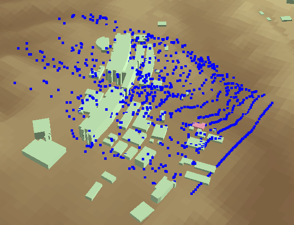
アニメーション表示

Animation